小世界性——与同规模 ER 随机图比较

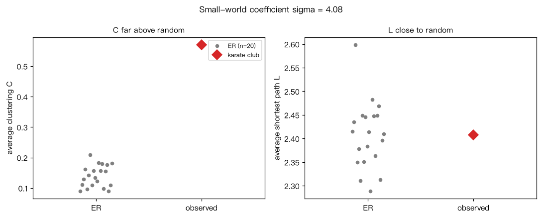
# 计算空手道网络的平均聚集系数 C 和平均最短路径 L；生成 20 个节点数、边数相同的 ER 随机图
# （取最大连通分支）得到 C_rand、L_rand；求小世界系数 sigma = (C/C_rand) / (L/L_rand)。
# 解读：C 远大于 C_rand 而 L 与 L_rand 接近时 sigma 明显大于 1，提示小世界性。
import networkx as nx
import numpy as np

G = nx.karate_club_graph()
n, m = G.number_of_nodes(), G.number_of_edges()
C, L = nx.average_clustering(G), nx.average_shortest_path_length(G)

C_rand, L_rand = [], []
for s in range(20):
    R = nx.gnm_random_graph(n, m, seed=s)
    R = R.subgraph(max(nx.connected_components(R), key=len)).copy()
    C_rand.append(nx.average_clustering(R))
    L_rand.append(nx.average_shortest_path_length(R))

sigma = (C / np.mean(C_rand)) / (L / np.mean(L_rand))
print(f"C = {C:.3f}（ER 均值 {np.mean(C_rand):.3f}）；L = {L:.3f}（ER 均值 {np.mean(L_rand):.3f}）；sigma = {sigma:.2f}")

# 作图：C 与 L 的真实值和 20 个 ER 随机图的取值
import matplotlib.pyplot as plt
fig, ax = plt.subplots(1, 2, figsize=(10, 4))
for a, obs, null, nm in [(ax[0], C, C_rand, "average clustering C"), (ax[1], L, L_rand, "average shortest path L")]:
    a.plot(np.linspace(-0.15, 0.15, 20), null, "o", color="0.5", ms=4, label="ER (n=20)")
    a.plot(1, obs, "D", color="C3", ms=9, label="karate club")
    a.set_xticks([0, 1]); a.set_xticklabels(["ER", "observed"]); a.set_xlim(-0.6, 1.6); a.set_ylabel(nm)
ax[0].legend(fontsize=8); ax[0].set_title("C far above random", fontsize=10)
ax[1].set_title("L close to random", fontsize=10)
fig.suptitle(f"Small-world coefficient sigma = {sigma:.2f}", fontsize=11)
plt.tight_layout(); plt.show()