Example07 / 09
大规模网络的计算策略——稀疏矩阵、近似介数与抽样偏倚
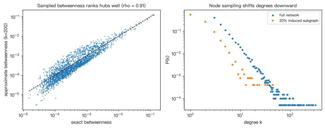
(a)2 万节点的 BA 网络:比较稠密与 CSR 稀疏矩阵的内存,用 scipy.sparse.csgraph 求连通分支、 用 scipy.sparse.linalg.eigsh 求最大特征值;(b)在 2000 节点网络上比较精确介数与 k 个源点抽样的近似介数 (Spearman 秩相关与前 20 名重合数、耗时);(c)随机抽取 20% 节点得到诱导子图,平均度与最大度如何变化。 解读:稀疏存储的内存与边数成正比;抽样介数对“前几名”的排序通常已足够稳定; 诱导子图的度会按抽样比例整体缩小,由子图估计的度分布不能直接代表全网络。
Output输出图
Output文字输出
(a) N=20000, M=59991;稠密矩阵约 3200 MB,CSR 约 2.08 MB
    最大度 323,连通分支 1 个,邻接矩阵最大特征值 21.86
(b) k= 50:耗时 0.10s(精确 4.19s),Spearman ρ = 0.860,前20名重合 14/20
(b) k=200:耗时 0.40s(精确 4.19s),Spearman ρ = 0.911,前20名重合 19/20
(c) 全网络:平均度 6.00,最大度 323;20% 节点诱导子图:平均度 1.22,最大度 45,孤立点 1468 个Code代码
# (a)2 万节点的 BA 网络:比较稠密与 CSR 稀疏矩阵的内存,用 scipy.sparse.csgraph 求连通分支、
#     用 scipy.sparse.linalg.eigsh 求最大特征值;(b)在 2000 节点网络上比较精确介数与 k 个源点抽样的近似介数
#     (Spearman 秩相关与前 20 名重合数、耗时);(c)随机抽取 20% 节点得到诱导子图,平均度与最大度如何变化。
# 解读:稀疏存储的内存与边数成正比;抽样介数对“前几名”的排序通常已足够稳定;
# 诱导子图的度会按抽样比例整体缩小,由子图估计的度分布不能直接代表全网络。
import time
import numpy as np
import scipy.sparse as sp
import scipy.sparse.csgraph as csg
import scipy.sparse.linalg as sla
from scipy.stats import spearmanr
import networkx as nx

# (a) 稀疏矩阵
G = nx.barabasi_albert_graph(20000, 3, seed=1)
A = nx.to_scipy_sparse_array(G, format="csr", dtype=np.float64)
dense_mb = G.number_of_nodes() ** 2 * 8 / 1e6
sparse_mb = (A.data.nbytes + A.indices.nbytes + A.indptr.nbytes) / 1e6
print("(a) N=%d, M=%d;稠密矩阵约 %.0f MB,CSR 约 %.2f MB" % (G.number_of_nodes(), G.number_of_edges(), dense_mb, sparse_mb))
deg = np.asarray(A.sum(axis=1)).ravel()
ncomp, labels = csg.connected_components(A, directed=False)
lam = sla.eigsh(A, k=1, which="LA", return_eigenvectors=False)[0]
print("    最大度 %d,连通分支 %d 个,邻接矩阵最大特征值 %.2f" % (deg.max(), ncomp, lam))

# (b) 近似介数
G2 = nx.barabasi_albert_graph(2000, 3, seed=2)
t0 = time.perf_counter(); bc = nx.betweenness_centrality(G2); t_exact = time.perf_counter() - t0
nodes = list(G2)
exact = np.array([bc[v] for v in nodes])
top_exact = set(np.argsort(-exact)[:20])
for k in (50, 200):
    t0 = time.perf_counter(); bck = nx.betweenness_centrality(G2, k=k, seed=0); t_k = time.perf_counter() - t0
    approx = np.array([bck[v] for v in nodes])
    rho = spearmanr(exact, approx).correlation
    overlap = len(top_exact & set(np.argsort(-approx)[:20]))
    print("(b) k=%3d:耗时 %.2fs(精确 %.2fs),Spearman ρ = %.3f,前20名重合 %d/20" % (k, t_k, t_exact, rho, overlap))

# (c) 节点抽样的诱导子图
rng = np.random.default_rng(3)
sub_nodes = rng.choice(G.number_of_nodes(), size=G.number_of_nodes() // 5, replace=False)
Gs = G.subgraph(sub_nodes)
d_full = np.array([d for _, d in G.degree()]); d_sub = np.array([d for _, d in Gs.degree()])
print("(c) 全网络:平均度 %.2f,最大度 %d;20%% 节点诱导子图:平均度 %.2f,最大度 %d,孤立点 %d 个" % (
    d_full.mean(), d_full.max(), d_sub.mean(), d_sub.max(), int((d_sub == 0).sum())))

# 作图:精确介数 vs 抽样近似介数(k=200);全网络与 20% 诱导子图的度分布
import matplotlib.pyplot as plt
fig, ax = plt.subplots(1, 2, figsize=(10, 4))
ax[0].loglog(exact[exact > 0], approx[exact > 0], ".", ms=3, alpha=0.5)
lim = [exact[exact > 0].min(), exact.max()]; ax[0].plot(lim, lim, "k--", lw=1)
ax[0].set_xlabel("exact betweenness"); ax[0].set_ylabel("approximate betweenness (k=200)")
ax[0].set_title(f"Sampled betweenness ranks hubs well (rho = {rho:.2f})", fontsize=10)
for dv, lab, mk in [(d_full, "full network", "o"), (d_sub[d_sub > 0], "20% induced subgraph", "s")]:
    v_, c_ = np.unique(dv, return_counts=True)
    ax[1].loglog(v_, c_ / c_.sum(), mk, ms=3, label=lab)
ax[1].set_xlabel("degree k"); ax[1].set_ylabel("P(k)"); ax[1].legend(fontsize=8)
ax[1].set_title("Node sampling shifts degrees downward", fontsize=10)
plt.tight_layout(); plt.show()Run在浏览器中运行
首次加载 Python 环境约需 20–40 秒;可以修改参数后重新运行。