Example06 / 11
关联矩阵、度矩阵与拉普拉斯矩阵
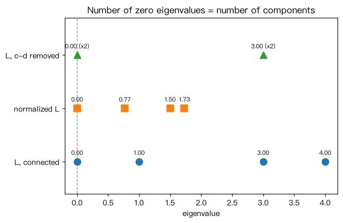
构造无定向关联矩阵 B、定向关联矩阵 ∇、度矩阵 D 与拉普拉斯矩阵 L = D − A,核对两个恒等式: B B^T = D + A,∇ ∇^T = L。再计算 L 的特征值(正文手算结果 0, 1, 3, 4)、归一化拉普拉斯的特征值, 并验证“零特征值的重数 = 连通分支数”:删去 c–d 后图分成两块,零特征值变为 2 个。
Output输出图
Output文字输出
关联矩阵 B(行 = 节点,列 = 边):
 [[1 1 0 0]
 [1 0 1 0]
 [0 1 1 1]
 [0 0 0 1]]
B B^T == D + A ? True
∇ ∇^T == L ? True
L =
 [[ 2 -1 -1  0]
 [-1  2 -1  0]
 [-1 -1  3 -1]
 [ 0  0 -1  1]]
L 的特征值: [-0.  1.  3.  4.]  之和 = 2M = 8
L x(x = (1,-1,0,0))= [ 3. -3.  0.  0.] → 特征值 3 的特征向量
二次型 x^T L x = 6.0 = Σ(x_i - x_j)^2 = 6.0
归一化拉普拉斯的特征值(落在 [0, 2]): [-0.      0.7713  1.5     1.7287]
删去 c–d 后 L 的特征值: [-0.  0.  3.  3.] ;零特征值个数 = 2 ;连通分支数 = 2
Code代码
# 构造无定向关联矩阵 B、定向关联矩阵 ∇、度矩阵 D 与拉普拉斯矩阵 L = D − A,核对两个恒等式:
# B B^T = D + A,∇ ∇^T = L。再计算 L 的特征值(正文手算结果 0, 1, 3, 4)、归一化拉普拉斯的特征值,
# 并验证“零特征值的重数 = 连通分支数”:删去 c–d 后图分成两块,零特征值变为 2 个。
import networkx as nx
import numpy as np

nodes = ["a", "b", "c", "d"]
edges = [("a", "b"), ("a", "c"), ("b", "c"), ("c", "d")]
G = nx.Graph(edges)
A = nx.to_numpy_array(G, nodelist=nodes)
Dm = np.diag(A.sum(axis=1))
L = Dm - A

B = nx.incidence_matrix(G, nodelist=nodes, edgelist=edges, oriented=False).toarray()
Nab = nx.incidence_matrix(G, nodelist=nodes, edgelist=edges, oriented=True).toarray()
print("关联矩阵 B(行 = 节点,列 = 边):\n", B.astype(int))
print("B B^T == D + A ?", np.allclose(B @ B.T, Dm + A))
print("∇ ∇^T == L ?", np.allclose(Nab @ Nab.T, L))
print("L =\n", L.astype(int))
print("L 的特征值:", np.round(np.linalg.eigvalsh(L), 4), " 之和 = 2M =", int(np.trace(L)))

x = np.array([1.0, -1.0, 0.0, 0.0])
print("L x(x = (1,-1,0,0))=", L @ x, "→ 特征值 3 的特征向量")
print("二次型 x^T L x =", x @ L @ x, "= Σ(x_i - x_j)^2 =",
      sum((x[nodes.index(u)] - x[nodes.index(v)]) ** 2 for u, v in edges))

Ln = nx.normalized_laplacian_matrix(G, nodelist=nodes).toarray()
print("归一化拉普拉斯的特征值(落在 [0, 2]):", np.round(np.linalg.eigvalsh(Ln), 4))

G2 = G.copy()
G2.remove_edge("c", "d")
L2 = nx.laplacian_matrix(G2, nodelist=nodes).toarray()
ev2 = np.linalg.eigvalsh(L2)
print("删去 c–d 后 L 的特征值:", np.round(ev2, 4),
      ";零特征值个数 =", int(np.sum(np.isclose(ev2, 0))),
      ";连通分支数 =", nx.number_connected_components(G2))

# 作图:三组特征值谱,零特征值的个数 = 连通分支数
import matplotlib.pyplot as plt

fig, ax = plt.subplots(figsize=(6.4, 4.2))
spectra = [("L, connected", np.linalg.eigvalsh(L), "o"), ("normalized L", np.linalg.eigvalsh(Ln), "s"),
           ("L, c-d removed", ev2, "^")]
for row, (name, ev, mk) in enumerate(spectra):
    ax.scatter(ev, [row] * len(ev), marker=mk, s=80, label=name, zorder=3)
    vals, mult = np.unique(np.round(np.abs(ev), 2), return_counts=True)
    for e, m in zip(vals, mult):
        ax.annotate("%.2f" % e + (" (x%d)" % m if m > 1 else ""), (e, row), textcoords="offset points",
                    xytext=(0, 9), ha="center", fontsize=8)
ax.axvline(0, color="0.6", ls="--", lw=1)
ax.set_yticks(range(3)); ax.set_yticklabels([s[0] for s in spectra]); ax.set_ylim(-0.6, 2.7)
ax.set_xlabel("eigenvalue")
ax.set_title("Number of zero eigenvalues = number of components")
plt.tight_layout(); plt.show()Run在浏览器中运行
首次加载 Python 环境约需 20–40 秒;可以修改参数后重新运行。