Example07 / 11
稀疏存储——边列表、CSR 与稠密矩阵的内存比较
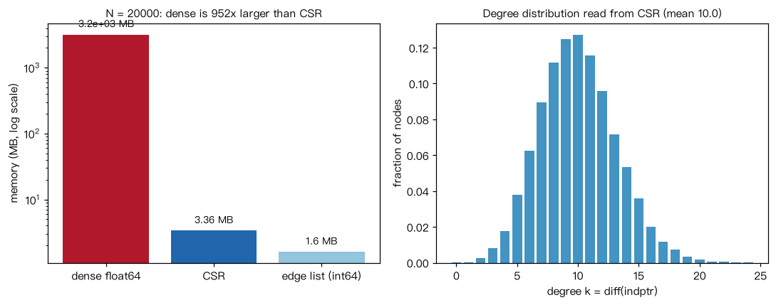
生成一个 N = 20000、平均度约 10 的随机稀疏网络(模拟一个蛋白质组规模的网络), 比较稠密 float64 邻接矩阵(只按 N^2 × 8 字节计算,不实际分配)与 CSR 稀疏矩阵的内存, 并展示 CSR 的三个数组如何直接给出邻居列表和度。 输出:密度约 5e-4;稠密矩阵约 3.2 GB,CSR 只有约 2–3 MB;indptr 差分即为度。
Output输出图
Output文字输出
N = 20000, M = 100000, 密度 = 5.00e-04
稠密矩阵约需 3.2 GB;CSR 实际占用 3.36 MB(952 倍差距)
节点 0 的邻居(来自 CSR): [1617, 4381, 9171, 9925, 13757, 16874, 17813]
NetworkX 给出的邻居:       [1617, 4381, 9171, 9925, 13757, 16874, 17813]
CSR 中 indptr 的差分就是度:与 NetworkX 一致吗? True
手工 CSR 与 SciPy CSR 相同吗? True
Code代码
# 生成一个 N = 20000、平均度约 10 的随机稀疏网络(模拟一个蛋白质组规模的网络),
# 比较稠密 float64 邻接矩阵(只按 N^2 × 8 字节计算,不实际分配)与 CSR 稀疏矩阵的内存,
# 并展示 CSR 的三个数组如何直接给出邻居列表和度。
# 输出:密度约 5e-4;稠密矩阵约 3.2 GB,CSR 只有约 2–3 MB;indptr 差分即为度。
import networkx as nx
import numpy as np
import scipy.sparse as sp

N, k_mean = 20000, 10
G = nx.gnm_random_graph(N, N * k_mean // 2, seed=1)
M = G.number_of_edges()
print("N = %d, M = %d, 密度 = %.2e" % (N, M, nx.density(G)))

S = nx.to_scipy_sparse_array(G, format="csr", dtype=np.float64)
dense_bytes = N * N * 8
csr_bytes = S.data.nbytes + S.indices.nbytes + S.indptr.nbytes
print("稠密矩阵约需 %.1f GB;CSR 实际占用 %.2f MB(%.0f 倍差距)"
      % (dense_bytes / 1e9, csr_bytes / 1e6, dense_bytes / csr_bytes))

i = 0
nbrs = S.indices[S.indptr[i]:S.indptr[i + 1]]
print("节点 0 的邻居(来自 CSR):", sorted(nbrs.tolist()))
print("NetworkX 给出的邻居:      ", sorted(G.neighbors(0)))
deg_csr = np.diff(S.indptr)
print("CSR 中 indptr 的差分就是度:与 NetworkX 一致吗?",
      np.array_equal(deg_csr, np.array([d for _, d in sorted(G.degree())])))

# 手工从边列表构造 CSR(正文“算法 3”),与 SciPy 的结果比较
u = np.array([e[0] for e in G.edges()] + [e[1] for e in G.edges()])
v = np.array([e[1] for e in G.edges()] + [e[0] for e in G.edges()])
count = np.bincount(u, minlength=N)
indptr = np.concatenate([[0], np.cumsum(count)])
pos = indptr[:-1].copy()
indices = np.empty(len(u), dtype=np.int64)
for a, b in zip(u, v):
    indices[pos[a]] = b
    pos[a] += 1
S2 = sp.csr_array((np.ones(len(u)), indices, indptr), shape=(N, N))
print("手工 CSR 与 SciPy CSR 相同吗?", (abs(S2 - S)).sum() == 0)

# 作图:左为三种存储方式的内存(对数轴),右为从 CSR 的 indptr 差分得到的度分布
import matplotlib.pyplot as plt

edge_bytes = 2 * M * 8                      # 边列表:每条边两个 int64
fig, (ax1, ax2) = plt.subplots(1, 2, figsize=(10, 4))
mem = {"dense float64": dense_bytes, "CSR": csr_bytes, "edge list (int64)": edge_bytes}
ax1.bar(list(mem), [b / 1e6 for b in mem.values()], color=["#b2182b", "#2166ac", "#92c5de"])
ax1.set_yscale("log"); ax1.set_ylabel("memory (MB, log scale)")
for i, b in enumerate(mem.values()):
    ax1.text(i, b / 1e6 * 1.3, "%.3g MB" % (b / 1e6), ha="center", fontsize=9)
ax1.set_title("N = %d: dense is %.0fx larger than CSR" % (N, dense_bytes / csr_bytes), fontsize=10)
ks, cnt = np.unique(deg_csr, return_counts=True)
ax2.bar(ks, cnt / N, color="#4393c3")
ax2.set_xlabel("degree k = diff(indptr)"); ax2.set_ylabel("fraction of nodes")
ax2.set_title("Degree distribution read from CSR (mean %.1f)" % deg_csr.mean(), fontsize=10)
plt.tight_layout(); plt.show()Run在浏览器中运行
首次加载 Python 环境约需 20–40 秒;可以修改参数后重新运行。