Example05 / 10
配置模型——从给定度序列生成随机网络
先从离散幂律(γ=2.5,k_min=2)抽取 N=5000 个节点的度序列,再用
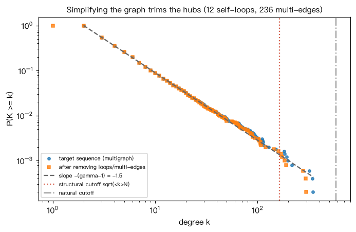
nx.configuration_model 随机配对“半边”。 检查三件事:(1)
配对产生的自环与重边数目(集中在枢纽上);(2) 化为简单图后度序列的改变;
(3) Molloy–Reed 判据 <k^2> - 2
Output输出图
Output文字输出
度序列: N=5000, <k>=5.30, k_max=348, 自然截断估计 k_min*N^(1/(γ-1))=585
配对后: 自环 12 条, 重边(多余的平行边)236 条
化为简单图后: <k>=5.20, k_max=299(原为 348)
Molloy–Reed: <k^2>-2<k> = 187.9  (>0 则存在巨连通分支)
巨连通分支占比 = 1.000
朋友悖论: 节点平均度 <k>=5.30, 边末端平均度 <k^2>/<k>=37.47
聚集系数: 模拟 C=0.0205, 配置模型近似 (<k^2>-<k>)^2/(<k>^3 N)=0.0502
结构截断 sqrt(<k>N)=163:k_max 超过它时,枢纽之间会被迫出现重边,删重边后近似公式高估 C
Code代码
# 先从离散幂律(γ=2.5,k_min=2)抽取 N=5000 个节点的度序列,再用 nx.configuration_model 随机配对“半边”。
# 检查三件事:(1) 配对产生的自环与重边数目(集中在枢纽上);(2) 化为简单图后度序列的改变;
# (3) Molloy–Reed 判据 <k^2> - 2<k> > 0 与巨连通分支的大小;并验证“朋友悖论”:随机一条边末端的平均度 <k^2>/<k> 远大于 <k>。
# 输出:自环与重边共有数百条且集中在枢纽,删除后最大度明显下降;判据为正,巨分支覆盖几乎全部节点;
#       由于 k_max 超过结构截断,C 的近似公式只给出数量级。
import networkx as nx
import numpy as np

rng = np.random.default_rng(0)
N, gamma, kmin = 5000, 2.5, 2
# 用连续幂律的逆变换抽样后向下取整,得到近似离散幂律的度序列
u = rng.random(N)
deg = np.floor(kmin * (1 - u) ** (-1 / (gamma - 1))).astype(int)
if deg.sum() % 2 == 1:          # 半边总数必须为偶数
    deg[0] += 1
print("度序列: N=%d, <k>=%.2f, k_max=%d, 自然截断估计 k_min*N^(1/(γ-1))=%.0f"
      % (N, deg.mean(), deg.max(), kmin * N ** (1 / (gamma - 1))))

M = nx.configuration_model(deg.tolist(), seed=1)          # MultiGraph,允许自环与重边
n_self = nx.number_of_selfloops(M)
n_multi = M.number_of_edges() - nx.Graph(M).number_of_edges()
print("配对后: 自环 %d 条, 重边(多余的平行边)%d 条" % (n_self, n_multi))

G = nx.Graph(M)                                           # 合并重边
G.remove_edges_from(nx.selfloop_edges(G))                 # 删除自环
deg_simple = np.array([d for _, d in G.degree()])
print("化为简单图后: <k>=%.2f, k_max=%d(原为 %d)" % (deg_simple.mean(), deg_simple.max(), deg.max()))

k1, k2 = deg.mean(), (deg.astype(float) ** 2).mean()
print("Molloy–Reed: <k^2>-2<k> = %.1f  (>0 则存在巨连通分支)" % (k2 - 2 * k1))
giant = max(nx.connected_components(G), key=len)
print("巨连通分支占比 = %.3f" % (len(giant) / N))
print("朋友悖论: 节点平均度 <k>=%.2f, 边末端平均度 <k^2>/<k>=%.2f" % (k1, k2 / k1))
C_theory = (k2 - k1) ** 2 / (k1 ** 3 * N)
print("聚集系数: 模拟 C=%.4f, 配置模型近似 (<k^2>-<k>)^2/(<k>^3 N)=%.4f" % (nx.transitivity(G), C_theory))
print("结构截断 sqrt(<k>N)=%.0f:k_max 超过它时,枢纽之间会被迫出现重边,删重边后近似公式高估 C" % np.sqrt(k1 * N))

# 作图:配对前后度分布的 CCDF,竖线为结构截断与自然截断
import matplotlib.pyplot as plt

fig, ax = plt.subplots(figsize=(6.4, 4.2))
for d, mk, lab in [(deg, "o", "target sequence (multigraph)"), (deg_simple, "s", "after removing loops/multi-edges")]:
    xs = np.sort(np.unique(d))
    ax.loglog(xs, [(d >= x).mean() for x in xs], mk, ms=3.5, alpha=0.8, label=lab)
xs = np.logspace(np.log10(kmin), np.log10(deg.max()), 50)
ax.loglog(xs, (xs / kmin) ** (1 - gamma), "--", color="0.4", label="slope -(gamma-1) = %.1f" % (1 - gamma))
ax.axvline(np.sqrt(k1 * N), color="#d6604d", ls=":", label="structural cutoff sqrt(<k>N)")
ax.axvline(kmin * N ** (1 / (gamma - 1)), color="0.6", ls="-.", label="natural cutoff")
ax.set_xlabel("degree k"); ax.set_ylabel("P(K >= k)"); ax.legend(fontsize=7)
ax.set_title("Simplifying the graph trims the hubs (%d self-loops, %d multi-edges)" % (n_self, n_multi), fontsize=10)
plt.tight_layout(); plt.show()Run在浏览器中运行
首次加载 Python 环境约需 20–40 秒;可以修改参数后重新运行。