功能连接指纹识别与差异可识别性

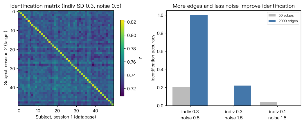
# 模拟 50 名被试、各两次扫描（session 1/2）。每人的 FC = 群体共同模式 + 个体特异模式 + 扫描噪声。
# 识别：对 session 2 的每个人，在 session 1 的“数据库”中找边向量相关最高的人，命中即识别正确（Finn 等, 2015 的思路）。
# 差异可识别性 I_diff = 同一人跨扫描相关的均值 − 不同人之间相关的均值（Amico & Goñi, 2018）。
# 输出解读：个体特异成分越强、使用的边越多，识别率和 I_diff 越高；
# 只用少量边或扫描噪声大（扫描时间短）时识别率下降。识别率高说明个体差异稳定，不等于这些差异与行为有关。
import numpy as np

rng = np.random.default_rng(7)                # 模拟数据，仅用于演示方法
N_sub, n_edge = 50, 2000
group = rng.standard_normal(n_edge)

def simulate(indiv_sd, noise_sd):
    indiv = indiv_sd * rng.standard_normal((N_sub, n_edge))
    s1 = group + indiv + noise_sd * rng.standard_normal((N_sub, n_edge))
    s2 = group + indiv + noise_sd * rng.standard_normal((N_sub, n_edge))
    return s1, s2

def identify(s1, s2, edges):
    a = s1[:, edges]; b = s2[:, edges]
    a = (a - a.mean(1, keepdims=True)) / a.std(1, keepdims=True)
    b = (b - b.mean(1, keepdims=True)) / b.std(1, keepdims=True)
    Cm = b @ a.T / len(edges)                 # 行：目标被试；列：数据库被试
    acc = np.mean(Cm.argmax(1) == np.arange(N_sub))
    i_self = np.mean(np.diag(Cm))
    i_other = (Cm.sum() - np.trace(Cm)) / (N_sub * (N_sub - 1))
    return acc, i_self - i_other

print("个体成分SD  扫描噪声SD  使用边数  识别率  I_diff")
acc_list = []                                 # 记录识别率，供作图
for indiv_sd, noise_sd in [(0.3, 0.5), (0.3, 1.5), (0.1, 1.5)]:
    s1, s2 = simulate(indiv_sd, noise_sd)
    for m in [50, 2000]:
        edges = rng.choice(n_edge, m, replace=False)
        acc, idiff = identify(s1, s2, edges)
        acc_list.append(acc)
        print(f"   {indiv_sd:.1f}        {noise_sd:.1f}       {m:5d}    {acc:.2f}   {idiff:.3f}")

import matplotlib.pyplot as plt
s1, s2 = simulate(0.3, 0.5)                   # 另抽一组数据画识别矩阵（全部边）
a = (s1 - s1.mean(1, keepdims=True)) / s1.std(1, keepdims=True)
b = (s2 - s2.mean(1, keepdims=True)) / s2.std(1, keepdims=True)
Cm = b @ a.T / n_edge
fig, axes = plt.subplots(1, 2, figsize=(10, 4))
im = axes[0].imshow(Cm, cmap="viridis")
fig.colorbar(im, ax=axes[0], shrink=0.8, label="r")
axes[0].set(xlabel="Subject, session 1 (database)", ylabel="Subject, session 2 (target)",
            title="Identification matrix (indiv SD 0.3, noise 0.5)")
acc_arr = np.array(acc_list).reshape(3, 2)
pos = np.arange(3)
axes[1].bar(pos - 0.2, acc_arr[:, 0], 0.4, color="#BBBBBB", label="50 edges")
axes[1].bar(pos + 0.2, acc_arr[:, 1], 0.4, color="#4477AA", label="2000 edges")
axes[1].set_xticks(pos, ["indiv 0.3\nnoise 0.5", "indiv 0.3\nnoise 1.5", "indiv 0.1\nnoise 1.5"])
axes[1].set(ylabel="Identification accuracy", ylim=(0, 1.05), title="More edges and less noise improve identification")
axes[1].legend(fontsize=8)
plt.tight_layout(); plt.show()