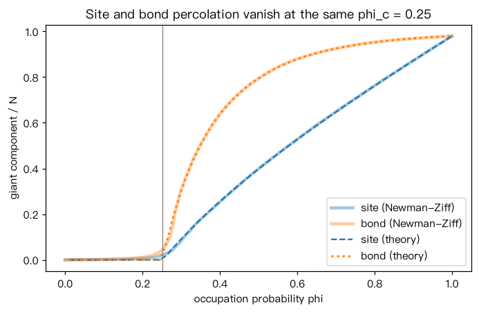
生成函数求解点渗流与边渗流，并与 Newman–Ziff 模拟比较

# 对给定度分布，点渗流（每个节点以概率 phi 保留）：u = 1 - phi + phi*G1(u)，S = phi*(1 - G0(u))；
# 边渗流（每条边以概率 phi 保留）：u = 1 - phi + phi*G1(u)，S = 1 - G0(u)。两者阈值相同：phi_c = <k>/(<k^2>-<k>)。
# 模拟用 Newman–Ziff 算法：按随机顺序逐个"加回"节点（或边），用并查集维护最大分支，一次得到整条曲线。
# 解读：理论曲线与模拟吻合；点渗流曲线始终低于边渗流曲线（删一个点等于删掉它的全部边），但两者在同一 phi_c 处消失。
import numpy as np
import networkx as nx

def moments_G(degs):
    k = np.arange(degs.max() + 1)
    P = np.bincount(degs, minlength=len(k)) / len(degs)
    G0 = lambda x: np.sum(P * x ** k)
    mk = np.sum(k * P)
    G1 = lambda x: np.sum(k[1:] * P[1:] * x ** (k[1:] - 1)) / mk
    return P, k, G0, G1

def solve_u(G1, phi, iters=2000):
    u = 0.0                                   # 从 0 开始迭代，收敛到最小非平凡解
    for _ in range(iters):
        u = 1 - phi + phi * G1(u)
    return u

def newman_ziff(G, mode="site", reps=20, seed=0):
    rng = np.random.default_rng(seed)
    nodes = list(G.nodes()); N = len(nodes); edges = list(G.edges())
    out = np.zeros(N + 1 if mode == "site" else len(edges) + 1)
    for _ in range(reps):
        parent = {v: v for v in nodes}; size = {v: 1 for v in nodes}
        def find(x):
            while parent[x] != x:
                parent[x] = parent[parent[x]]; x = parent[x]
            return x
        def union(a, b, smax):
            ra, rb = find(a), find(b)
            if ra != rb:
                if size[ra] < size[rb]: ra, rb = rb, ra
                parent[rb] = ra; size[ra] += size[rb]; smax = max(smax, size[ra])
            return smax
        curve = [0]; smax = 0
        if mode == "site":
            present = set()
            for v in rng.permutation(N):
                v = nodes[v]; present.add(v); smax = max(smax, 1)
                for w in G[v]:
                    if w in present: smax = union(v, w, smax)
                curve.append(smax)
        else:
            smax = 1
            for e in rng.permutation(len(edges)):
                a, b = edges[e]; smax = union(a, b, smax); curve.append(smax)
        out += np.array(curve) / N
    return out / reps

G = nx.gnp_random_graph(5000, 4 / 4999, seed=1)
degs = np.array([d for _, d in G.degree()])
P, k, G0, G1 = moments_G(degs)
phi_c = degs.mean() / (np.mean(degs ** 2) - degs.mean())
print("ER <k>=%.2f  理论 phi_c = %.3f (即随机删除临界比例 f_c = %.3f)" % (degs.mean(), phi_c, 1 - phi_c))
site = newman_ziff(G, "site"); bond = newman_ziff(G, "bond")
for phi in [0.2, 0.3, 0.5, 0.8]:
    u = solve_u(G1, phi)
    S_site, S_bond = phi * (1 - G0(u)), 1 - G0(u)
    s_sim = site[int(phi * G.number_of_nodes())]; b_sim = bond[int(phi * G.number_of_edges())]
    print("phi=%.1f  点渗流 理论 %.3f 模拟 %.3f | 边渗流 理论 %.3f 模拟 %.3f" % (phi, S_site, s_sim, S_bond, b_sim))

import matplotlib.pyplot as plt
phis = np.linspace(0.01, 1, 60)
S_th = np.array([1 - G0(solve_u(G1, ph, iters=500)) for ph in phis])
fig, ax = plt.subplots(figsize=(6.4, 4.2))
ax.plot(np.arange(len(site)) / G.number_of_nodes(), site, c="tab:blue", lw=3, alpha=0.4, label="site (Newman-Ziff)")
ax.plot(np.arange(len(bond)) / G.number_of_edges(), bond, c="tab:orange", lw=3, alpha=0.4, label="bond (Newman-Ziff)")
ax.plot(phis, phis * S_th, "--", c="tab:blue", label="site (theory)")
ax.plot(phis, S_th, ":", c="tab:orange", lw=2, label="bond (theory)")
ax.axvline(phi_c, c="0.5", lw=0.8)
ax.set_xlabel("occupation probability phi"); ax.set_ylabel("giant component / N"); ax.legend()
ax.set_title("Site and bond percolation vanish at the same phi_c = %.2f" % phi_c)
plt.tight_layout(); plt.show()