Example09 / 12
可观测性——根强连通分支与最少观测节点
Liu、Slotine 与 Barabási(2013):画推断图(若 x_j 出现在 x_i 的方程中,则连 x_i -> x_j), 分解为强连通分支(SCC);没有入边的“根 SCC”每个至少要放一个观测节点——这是任何(非线性)系统可观测的必要条件。 线性系统可借助对偶性:(A, C) 可观测 <=> (A^T, C^T) 可控,所以最少观测节点数 = 反向网络的最少驱动节点数。 解读:根 SCC 个数是下界;线性系统的充分观测集合通常更大(还要消除“扩张”)。
Output输出图
Output文字输出
根 SCC 个数(任意动力学的必要观测节点数)= 44
线性动力学的最少观测节点数(对偶:反向图最大匹配)= 68
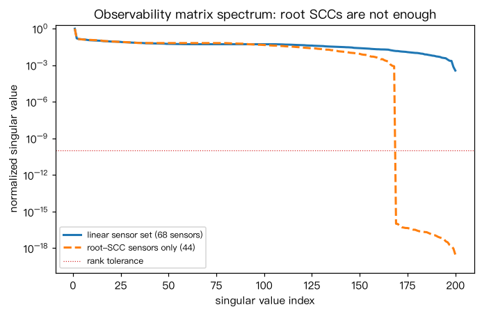
线性观测集合的可观测性秩 = 200 / 200
只放根 SCC 观测节点时的线性可观测性秩 = 168 / 200(不足说明线性系统需要更多观测)
Code代码
# Liu、Slotine 与 Barabási(2013):画推断图(若 x_j 出现在 x_i 的方程中,则连 x_i -> x_j),
# 分解为强连通分支(SCC);没有入边的“根 SCC”每个至少要放一个观测节点——这是任何(非线性)系统可观测的必要条件。
# 线性系统可借助对偶性:(A, C) 可观测 <=> (A^T, C^T) 可控,所以最少观测节点数 = 反向网络的最少驱动节点数。
# 解读:根 SCC 个数是下界;线性系统的充分观测集合通常更大(还要消除“扩张”)。
import numpy as np
import networkx as nx

def matching_drivers(G):
    Bg = nx.Graph()
    top = [("o", u) for u in G]
    Bg.add_nodes_from(top); Bg.add_nodes_from([("i", v) for v in G])
    Bg.add_edges_from((("o", u), ("i", v)) for u, v in G.edges())
    M = nx.bipartite.hopcroft_karp_matching(Bg, top_nodes=top)
    D = [v for v in G if ("i", v) not in M]
    return D if D else [next(iter(G))]

# 系统有向图 S:u -> v 表示 u 影响 v(u 出现在 v 的方程中);推断图 = S 的反向图
S = nx.gnm_random_graph(200, 300, directed=True, seed=5)
inference = S.reverse(copy=True)
cond = nx.condensation(inference)
root_sccs = [c for c in cond if cond.in_degree(c) == 0]
sensors_lower = [min(cond.nodes[c]["members"]) for c in root_sccs]     # 每个根 SCC 任取一个节点
sensors_linear = matching_drivers(inference)                            # 线性情形:反向图上的驱动节点
print("根 SCC 个数(任意动力学的必要观测节点数)= %d" % len(root_sccs))
print("线性动力学的最少观测节点数(对偶:反向图最大匹配)= %d" % len(sensors_linear))

# 用 Kalman 可观测性矩阵在随机权重下检验线性观测集合
n = S.number_of_nodes()
rng = np.random.default_rng(0)
A = np.zeros((n, n))
for u, v in S.edges():
    A[v, u] = rng.uniform(0.5, 1.5)
A /= max(1.0, np.abs(np.linalg.eigvals(A)).max())
C = np.zeros((len(sensors_linear), n)); C[np.arange(len(sensors_linear)), sensors_linear] = 1.0
blocks, X = [], C.copy()
for _ in range(n):
    blocks.append(X); X = X @ A
O = np.vstack(blocks)
s = np.linalg.svd(O, compute_uv=False)
print("线性观测集合的可观测性秩 = %d / %d" % (int((s > 1e-10 * s[0]).sum()), n))
C2 = np.zeros((len(sensors_lower), n)); C2[np.arange(len(sensors_lower)), sensors_lower] = 1.0
blocks, X = [], C2.copy()
for _ in range(n):
    blocks.append(X); X = X @ A
s2 = np.linalg.svd(np.vstack(blocks), compute_uv=False)
print("只放根 SCC 观测节点时的线性可观测性秩 = %d / %d(不足说明线性系统需要更多观测)"
      % (int((s2 > 1e-10 * s2[0]).sum()), n))

import matplotlib.pyplot as plt
fig, ax = plt.subplots(figsize=(6.4, 4.2))
ax.semilogy(np.arange(1, len(s) + 1), s / s[0], "-", lw=2, label="linear sensor set (%d sensors)" % len(sensors_linear))
ax.semilogy(np.arange(1, len(s2) + 1), np.maximum(s2 / s2[0], 1e-20), "--", lw=2,
            label="root-SCC sensors only (%d)" % len(sensors_lower))
ax.axhline(1e-10, c="tab:red", lw=0.8, ls=":", label="rank tolerance")
ax.set_ylim(1e-20, 2); ax.set_xlabel("singular value index"); ax.set_ylabel("normalized singular value")
ax.legend(fontsize=8); ax.set_title("Observability matrix spectrum: root SCCs are not enough")
plt.tight_layout(); plt.show()Run在浏览器中运行
首次加载 Python 环境约需 20–40 秒;可以修改参数后重新运行。