多元宇宙分析——把所有合理的网络构建选择组合起来同时报告

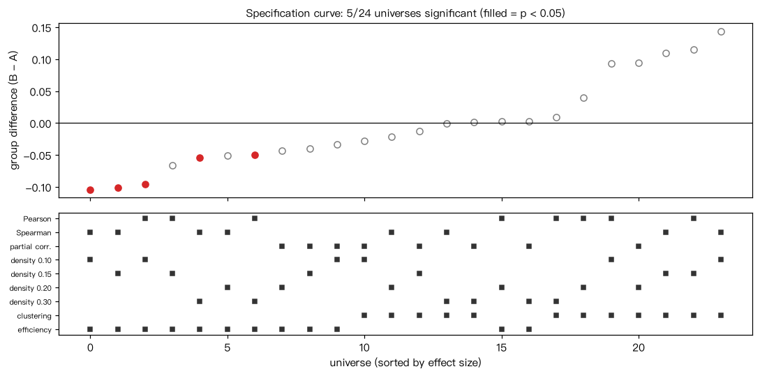
# 模拟两组被试（各 60 人、30 个节点），B 组只在一个 6 节点子模块内的连接略强（真实差异很小）。
# 分析选择的组合（共 3×4×2 = 24 个“宇宙”）：边的统计量（Pearson、Spearman、偏相关）×
# 网络密度（10%、15%、20%、30%）× 指标（平均聚集系数、全局效率）。
# 每个宇宙用 200 次组标签置换计算 p 值，最后按效应量排序，打印“设定曲线”（specification curve）
# 并统计显著宇宙所占比例。
# 解读：结论在不同宇宙中的一致程度本身就是结果。在这组模拟数据中，效应的方向和显著性都随边的统计量、
# 密度和指标而变；若只挑其中显著的一个宇宙报告，就是挑选性报告。
# 置换检验要在“整条流水线”外层做：每次置换都重新计算相关、阈值化和指标。
import itertools
import numpy as np
import networkx as nx
from scipy.stats import rankdata

rng = np.random.default_rng(2026)
n_nodes, n_per_group = 30, 60

def simulate_group(n, boost, rng):
    """单因子背景 + 子模块 0–5 共享额外因子（强度 boost）。模拟数据。"""
    g = rng.normal(size=(n, 1)); m = rng.normal(size=(n, 1))
    X = 0.5 * g + rng.normal(size=(n, n_nodes))
    X[:, :6] += boost * m
    return X

XA = simulate_group(n_per_group, 0.5, rng)
XB = simulate_group(n_per_group, 0.8, rng)

def edge_matrix(X, kind):
    if kind == "pearson":
        return np.corrcoef(X.T)
    if kind == "spearman":
        return np.corrcoef(np.apply_along_axis(rankdata, 0, X).T)
    P = np.linalg.inv(np.cov(X.T))                       # 偏相关：由精度矩阵标准化得到
    d = np.sqrt(np.diag(P)); R = -P / np.outer(d, d); np.fill_diagonal(R, 1)
    return R

def graph_at_density(C, density):
    iu = np.triu_indices(C.shape[0], 1)
    keep = np.argsort(-np.abs(C[iu]))[:int(round(density * len(iu[0])))]
    G = nx.Graph(); G.add_nodes_from(range(C.shape[0])); G.add_edges_from(zip(iu[0][keep], iu[1][keep]))
    return G

metrics = {"clustering": nx.average_clustering, "efficiency": nx.global_efficiency}

def group_diff(XA, XB, kind, density, metric):
    f = metrics[metric]
    return f(graph_at_density(edge_matrix(XB, kind), density)) - f(graph_at_density(edge_matrix(XA, kind), density))

X_all = np.vstack([XA, XB]); n_perm = 200
results = []
for kind, dens, met in itertools.product(["pearson", "spearman", "partial"], [0.10, 0.15, 0.20, 0.30], metrics):
    obs = group_diff(XA, XB, kind, dens, met)
    null = []
    for _ in range(n_perm):
        idx = rng.permutation(len(X_all))
        null.append(group_diff(X_all[idx[:n_per_group]], X_all[idx[n_per_group:]], kind, dens, met))
    p = (1 + np.sum(np.abs(null) >= abs(obs))) / (n_perm + 1)
    results.append((obs, p, kind, dens, met))

results.sort(key=lambda r: r[0])
print("设定曲线（按效应量排序）：")
for obs, p, kind, dens, met in results:
    print(f"  {kind:8s} 密度 {dens:.2f} {met:10s} 差值 {obs:+.4f}  p = {p:.3f} {'*' if p < 0.05 else ''}")
sig = sum(r[1] < 0.05 for r in results)
print(f"显著宇宙：{sig}/{len(results)}；效应量中位数 {np.median([r[0] for r in results]):+.4f}；"
      f"效应为正的宇宙比例 {np.mean([r[0] > 0 for r in results]):.2f}")

# 作图：设定曲线（上：按效应量排序，实心 = p < 0.05；下：每个宇宙的分析选择）
import matplotlib.pyplot as plt
fig, ax = plt.subplots(2, 1, figsize=(10, 5), sharex=True, gridspec_kw={"height_ratios": [2, 1.4]})
x = np.arange(len(results))
for i, (obs, p, kind, dens, met) in enumerate(results):
    ax[0].plot(i, obs, "o", color="C3" if p < 0.05 else "0.5", mfc="C3" if p < 0.05 else "white")
ax[0].axhline(0, color="k", lw=0.8); ax[0].set_ylabel("group difference (B - A)")
ax[0].set_title(f"Specification curve: {sig}/{len(results)} universes significant (filled = p < 0.05)", fontsize=10)
rows = ["pearson", "spearman", "partial", "0.1", "0.15", "0.2", "0.3", "clustering", "efficiency"]
for i, (obs, p, kind, dens, met) in enumerate(results):
    for lab in (kind, f"{dens:g}", met):
        ax[1].plot(i, rows.index(lab), "s", color="0.2", ms=4)
ax[1].set_yticks(range(len(rows))); ax[1].set_yticklabels(["Pearson", "Spearman", "partial corr.", "density 0.10",
                                                           "density 0.15", "density 0.20", "density 0.30",
                                                           "clustering", "efficiency"], fontsize=7)
ax[1].invert_yaxis(); ax[1].set_xlabel("universe (sorted by effect size)")
plt.tight_layout(); plt.show()