Example11 / 15
多分辨率扫描与共识聚类
- 在空手道网络上扫描分辨率 γ,每个 γ 运行 Louvain 50 次,记录社团数的中位数与“划分稳定性” (50 个划分两两之间 ARI 的平均值);稳定性高的 γ 区间提示较稳健的尺度。
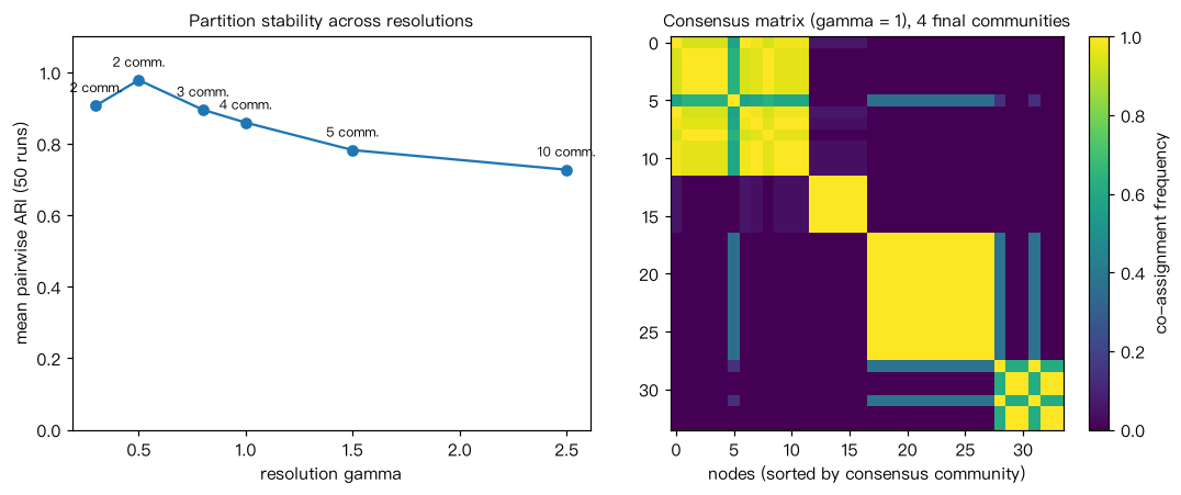
- 共识聚类(Lancichinetti 与 Fortunato 2012):在 γ=1 下运行 50 次,得到共识矩阵 D_ij = 节点 i、j 被分到同一社团的比例;删去 D_ij < τ(τ=0.5)的元素,以 D 为加权网络再运行 Louvain, 重复直到 D 只含 0 和 1。最终得到一个稳定的共识划分。 输出:(a) γ≈0.5 时划分最稳定(两个社团);γ 增大后社团变多、近似等价的划分增多,稳定性下降;
- 共识划分的社团数与 Q,以及各节点的“归属一致度”。
Output输出图
Output文字输出
(a) γ=0.3  社团数中位数 2  平均两两 ARI = 0.907
(a) γ=0.5  社团数中位数 2  平均两两 ARI = 0.978
(a) γ=0.8  社团数中位数 3  平均两两 ARI = 0.895
(a) γ=1.0  社团数中位数 4  平均两两 ARI = 0.859
(a) γ=1.5  社团数中位数 5  平均两两 ARI = 0.782
(a) γ=2.5  社团数中位数 10  平均两两 ARI = 0.727
(b) 迭代 1 轮后收敛:4 个社团,Q = 0.419
第一轮共识矩阵中归属一致度最低的 5 个节点: [9, 27, 23, 24, 25] [0.65, 0.75, 0.75, 0.87, 0.87]Code代码
# (a) 在空手道网络上扫描分辨率 γ,每个 γ 运行 Louvain 50 次,记录社团数的中位数与“划分稳定性”
#     (50 个划分两两之间 ARI 的平均值);稳定性高的 γ 区间提示较稳健的尺度。
# (b) 共识聚类(Lancichinetti 与 Fortunato 2012):在 γ=1 下运行 50 次,得到共识矩阵
#     D_ij = 节点 i、j 被分到同一社团的比例;删去 D_ij < τ(τ=0.5)的元素,以 D 为加权网络再运行 Louvain,
#     重复直到 D 只含 0 和 1。最终得到一个稳定的共识划分。
# 输出:(a) γ≈0.5 时划分最稳定(两个社团);γ 增大后社团变多、近似等价的划分增多,稳定性下降;
#       (b) 共识划分的社团数与 Q,以及各节点的“归属一致度”。
import itertools
import networkx as nx
import numpy as np


def ari(x, y):
    xs, xi = np.unique(x, return_inverse=True)
    ys, yi = np.unique(y, return_inverse=True)
    T = np.zeros((len(xs), len(ys)))
    np.add.at(T, (xi, yi), 1)
    c2 = lambda v: v * (v - 1) / 2
    s_ij, s_a, s_b, n2 = c2(T).sum(), c2(T.sum(1)).sum(), c2(T.sum(0)).sum(), c2(T.sum())
    e = s_a * s_b / n2
    den = 0.5 * (s_a + s_b) - e
    return 1.0 if den == 0 else (s_ij - e) / den


def labels(comms, n):
    lab = np.empty(n, int)
    for i, c in enumerate(comms):
        lab[list(c)] = i
    return lab


K = nx.karate_club_graph()
G = nx.Graph(K.edges())
n = G.number_of_nodes()

scan = []                                      # 存下结果用于作图
for gamma in [0.3, 0.5, 0.8, 1.0, 1.5, 2.5]:
    labs = [labels(nx.community.louvain_communities(G, resolution=gamma, seed=s), n) for s in range(50)]
    stab = np.mean([ari(a, b) for a, b in itertools.combinations(labs, 2)])
    scan.append((gamma, np.median([l.max() + 1 for l in labs]), stab))
    print("(a) γ=%.1f  社团数中位数 %d  平均两两 ARI = %.3f" % (gamma, np.median([l.max() + 1 for l in labs]), stab))


def consensus_matrix(H, runs=50, seed0=0):
    D = np.zeros((n, n))
    for s in range(runs):
        lab = labels(nx.community.louvain_communities(H, weight="weight", seed=seed0 + s), n)
        D += lab[:, None] == lab[None, :]
    return D / runs


D = consensus_matrix(G)
first = D.copy()
for it in range(20):
    if np.all((D == 0) | (D == 1)):
        break
    W = np.where(D >= 0.5, D, 0.0)
    np.fill_diagonal(W, 0)
    H = nx.from_numpy_array(W)
    D = consensus_matrix(H, seed0=100 * (it + 1))
comms = [set(c) for c in nx.connected_components(nx.from_numpy_array(np.where(D == 1, 1, 0) - np.eye(n)))]
print("(b) 迭代 %d 轮后收敛:%d 个社团,Q = %.3f" % (it, len(comms), nx.community.modularity(G, comms)))
lab = labels(comms, n)
agree = np.array([first[i, lab == lab[i]].mean() for i in range(n)])
print("    第一轮共识矩阵中归属一致度最低的 5 个节点:", np.argsort(agree)[:5].tolist(),
      np.round(np.sort(agree)[:5], 2).tolist())

# 作图:左为稳定性随 γ 的变化(标注社团数中位数);右为按共识划分排序的第一轮共识矩阵
import matplotlib.pyplot as plt

fig, (ax1, ax2) = plt.subplots(1, 2, figsize=(10, 4.2))
g_, nc_, st_ = zip(*scan)
ax1.plot(g_, st_, "o-")
for x, y, c_ in zip(g_, st_, nc_):
    ax1.annotate("%d comm." % c_, (x, y), textcoords="offset points", xytext=(0, 8), ha="center", fontsize=8)
ax1.set_xlabel("resolution gamma"); ax1.set_ylabel("mean pairwise ARI (50 runs)"); ax1.set_ylim(0, 1.1)
ax1.set_title("Partition stability across resolutions", fontsize=10)
order = np.argsort(lab, kind="stable")
im = ax2.imshow(first[np.ix_(order, order)], cmap="viridis", vmin=0, vmax=1)
fig.colorbar(im, ax=ax2, label="co-assignment frequency")
ax2.set_title("Consensus matrix (gamma = 1), %d final communities" % len(comms), fontsize=10)
ax2.set_xlabel("nodes (sorted by consensus community)")
plt.tight_layout(); plt.show()Run在浏览器中运行
首次加载 Python 环境约需 20–40 秒;可以修改参数后重新运行。