Example12 / 15
LFR 基准网络上的算法比较
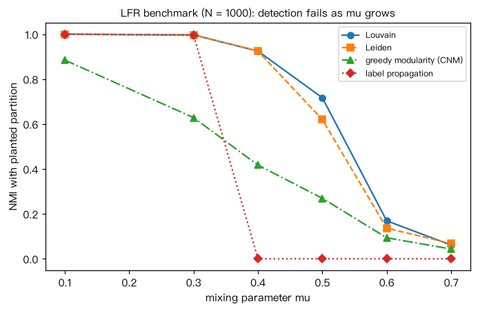
LFR 基准(Lancichinetti、Fortunato 与 Radicchi 2008)生成度分布与社团大小都服从幂律的网络, 混合参数 μ 为每个节点连向社团外部的边所占比例。μ 越大社团越难识别。 对 μ = 0.1–0.7 各生成网络,比较 Louvain、Leiden(模块度)、贪心模块度(CNM)、标签传播四种算法 与种植划分之间的 NMI。(NMI 采用算术平均归一化,与前面示例的定义相同。) 输出:μ≤0.3 时 Louvain、Leiden、标签传播的 NMI 接近 1,贪心模块度较早下降(倾向于合并小社团); 标签传播在 μ 较大时可能整体塌缩为一个社团(NMI=0);μ≥0.6 时所有算法都接近失效。 这里每个 μ 只生成一个网络、只用一个种子,数值会随种子波动,正式比较应多次重复取平均。
Output输出图
Output文字输出
μ     Louvain    Leiden     贪心模块度      标签传播
0.1     1.000     1.000     0.885     1.000
0.3     0.997     0.997     0.628     0.995
0.4     0.925     0.925     0.417     0.000
0.5     0.717     0.620     0.269     0.000
0.6     0.169     0.136     0.093     0.000
0.7     0.061     0.068     0.043     0.000
Code代码
# LFR 基准(Lancichinetti、Fortunato 与 Radicchi 2008)生成度分布与社团大小都服从幂律的网络,
# 混合参数 μ 为每个节点连向社团外部的边所占比例。μ 越大社团越难识别。
# 对 μ = 0.1–0.7 各生成网络,比较 Louvain、Leiden(模块度)、贪心模块度(CNM)、标签传播四种算法
# 与种植划分之间的 NMI。(NMI 采用算术平均归一化,与前面示例的定义相同。)
# 输出:μ≤0.3 时 Louvain、Leiden、标签传播的 NMI 接近 1,贪心模块度较早下降(倾向于合并小社团);
#       标签传播在 μ 较大时可能整体塌缩为一个社团(NMI=0);μ≥0.6 时所有算法都接近失效。
#       这里每个 μ 只生成一个网络、只用一个种子,数值会随种子波动,正式比较应多次重复取平均。
import networkx as nx
import numpy as np


def nmi(x, y):
    xs, xi = np.unique(x, return_inverse=True)
    ys, yi = np.unique(y, return_inverse=True)
    T = np.zeros((len(xs), len(ys)))
    np.add.at(T, (xi, yi), 1)
    P = T / T.sum()
    H = lambda p: -(p[p > 0] * np.log2(p[p > 0])).sum()
    hx, hy = H(P.sum(1)), H(P.sum(0))
    return 2 * (hx + hy - H(P.ravel())) / (hx + hy)


def labels(comms, nodes):
    lab = {v: i for i, c in enumerate(comms) for v in c}
    return np.array([lab[v] for v in nodes])


algos = {
    "Louvain": lambda G: nx.community.louvain_communities(G, seed=0),
    "Leiden": lambda G: nx.community.leiden_communities(G, metric="modularity", seed=0),
    "贪心模块度": lambda G: nx.community.greedy_modularity_communities(G),
    "标签传播": lambda G: nx.community.asyn_lpa_communities(G, seed=0),
}
print("μ    " + "  ".join("%8s" % a for a in algos))
table = []                                         # 存下结果用于作图
for mu in [0.1, 0.3, 0.4, 0.5, 0.6, 0.7]:
    G = nx.LFR_benchmark_graph(1000, 2.5, 1.5, mu, average_degree=20, max_degree=50,
                               min_community=20, max_community=100, seed=3)
    G.remove_edges_from(nx.selfloop_edges(G))
    nodes = list(G)
    truth_sets = {frozenset(G.nodes[v]["community"]) for v in G}
    truth = labels(truth_sets, nodes)
    row = [nmi(truth, labels(list(f(G)), nodes)) for f in algos.values()]
    print("%.1f  " % mu + "  ".join("%8.3f" % r for r in row))
    table.append([mu] + row)

# 作图:四种算法的 NMI 随混合参数 μ 的变化
import matplotlib.pyplot as plt

tb = np.array(table)
fig, ax = plt.subplots(figsize=(6.4, 4.2))
for j, (lab, mk) in enumerate(zip(["Louvain", "Leiden", "greedy modularity (CNM)", "label propagation"],
                                  ["o-", "s--", "^-.", "D:"])):
    ax.plot(tb[:, 0], tb[:, j + 1], mk, label=lab)
ax.set_xlabel("mixing parameter mu"); ax.set_ylabel("NMI with planted partition")
ax.set_ylim(-0.05, 1.05); ax.legend(fontsize=8)
ax.set_title("LFR benchmark (N = 1000): detection fails as mu grows", fontsize=10)
plt.tight_layout(); plt.show()Run在浏览器中运行
首次加载 Python 环境约需 20–40 秒;可以修改参数后重新运行。