Example07 / 15
随机块模型与可检测性阈值
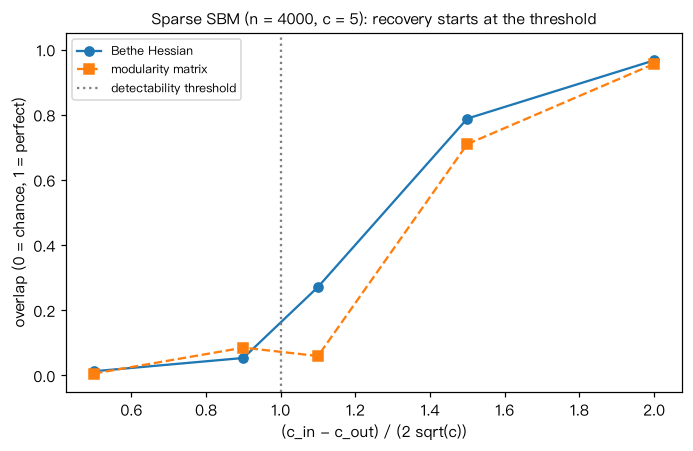
用两组等大的种植划分模型(planted partition SBM)生成稀疏网络:组内连边概率 c_in/n,组间 c_out/n, 平均度 c = (c_in + c_out)/2 固定为 5。理论(Decelle 等 2011)给出:当 |c_in - c_out| ≤ 2√c 时, 任何算法都无法以优于随机猜测的准确率恢复分组。这里用 Bethe Hessian 谱方法 H(r) = (r²-1)I - rA + D,r = √c(Saade 等 2014)与模块度矩阵谱二分恢复分组, 用“重叠度” overlap = 2·(正确比例) - 1(0 为随机猜测,1 为完全恢复)衡量。 输出:overlap 在阈值(Δc/2√c = 1)附近由约 0 开始上升;模块度谱方法在稀疏网络上通常更差。
Output输出图
Output文字输出
Δc/2√c = 0.5  (c_in=6.12, c_out=3.88)  overlap: Bethe Hessian 0.01, 模块度谱 0.01
Δc/2√c = 0.9  (c_in=7.01, c_out=2.99)  overlap: Bethe Hessian 0.05, 模块度谱 0.09
Δc/2√c = 1.1  (c_in=7.46, c_out=2.54)  overlap: Bethe Hessian 0.27, 模块度谱 0.06
Δc/2√c = 1.5  (c_in=8.35, c_out=1.65)  overlap: Bethe Hessian 0.79, 模块度谱 0.71
Δc/2√c = 2.0  (c_in=9.47, c_out=0.53)  overlap: Bethe Hessian 0.97, 模块度谱 0.96
Code代码
# 用两组等大的种植划分模型(planted partition SBM)生成稀疏网络:组内连边概率 c_in/n,组间 c_out/n,
# 平均度 c = (c_in + c_out)/2 固定为 5。理论(Decelle 等 2011)给出:当 |c_in - c_out| ≤ 2√c 时,
# 任何算法都无法以优于随机猜测的准确率恢复分组。这里用 Bethe Hessian 谱方法
# H(r) = (r²-1)I - rA + D,r = √c(Saade 等 2014)与模块度矩阵谱二分恢复分组,
# 用“重叠度” overlap = 2·(正确比例) - 1(0 为随机猜测,1 为完全恢复)衡量。
# 输出:overlap 在阈值(Δc/2√c = 1)附近由约 0 开始上升;模块度谱方法在稀疏网络上通常更差。
import networkx as nx
import numpy as np
import scipy.sparse as sp
from scipy.sparse.linalg import LinearOperator, eigsh

n, c = 4000, 5.0
half = n // 2
truth = np.r_[np.zeros(half, int), np.ones(half, int)]
thr = 2 * np.sqrt(c)


def overlap(labels):
    acc = (labels == truth).mean()
    return 2 * max(acc, 1 - acc) - 1


curve = []                                            # 存下结果用于作图
for ratio in [0.5, 0.9, 1.1, 1.5, 2.0]:
    dc = ratio * thr                                  # Δc = c_in - c_out
    c_in, c_out = c + dc / 2, c - dc / 2
    res_bh, res_mod = [], []
    for seed in range(3):
        G = nx.stochastic_block_model([half, half], [[c_in / n, c_out / n], [c_out / n, c_in / n]], seed=seed)
        A = nx.to_scipy_sparse_array(G, nodelist=range(n), format="csr", dtype=float)
        k = np.asarray(A.sum(1)).ravel()
        r = np.sqrt(k.mean())
        H = (r ** 2 - 1) * sp.identity(n) - r * A + sp.diags(k)
        vals, vecs = eigsh(H, k=2, which="SA")
        v = vecs[:, np.argsort(vals)[1]]               # 第二小特征值的特征向量
        res_bh.append(overlap((v > 0).astype(int)))
        # 模块度矩阵 B = A - k k^T/2m 的主特征向量(隐式矩阵乘法,不显式构造稠密 B)
        m2 = k.sum()
        Bop = LinearOperator((n, n), matvec=lambda x: A @ x - k * (k @ x) / m2, dtype=float)
        _, u = eigsh(Bop, k=1, which="LA")
        res_mod.append(overlap((u[:, 0] > 0).astype(int)))
    print("Δc/2√c = %.1f  (c_in=%.2f, c_out=%.2f)  overlap: Bethe Hessian %.2f, 模块度谱 %.2f"
          % (ratio, c_in, c_out, np.mean(res_bh), np.mean(res_mod)))
    curve.append((ratio, np.mean(res_bh), np.mean(res_mod)))

# 作图:overlap 随 Δc/2√c 的变化,竖线为可检测性阈值
import matplotlib.pyplot as plt

rs, ob, om = zip(*curve)
fig, ax = plt.subplots(figsize=(6.4, 4.2))
ax.plot(rs, ob, "o-", label="Bethe Hessian")
ax.plot(rs, om, "s--", label="modularity matrix")
ax.axvline(1, color="0.5", ls=":", label="detectability threshold")
ax.set_xlabel("(c_in - c_out) / (2 sqrt(c))"); ax.set_ylabel("overlap (0 = chance, 1 = perfect)")
ax.set_ylim(-0.05, 1.05); ax.legend(fontsize=8)
ax.set_title("Sparse SBM (n = %d, c = %.0f): recovery starts at the threshold" % (n, c), fontsize=10)
plt.tight_layout(); plt.show()Run在浏览器中运行
首次加载 Python 环境约需 20–40 秒;可以修改参数后重新运行。