边时间序列与高振幅共波动

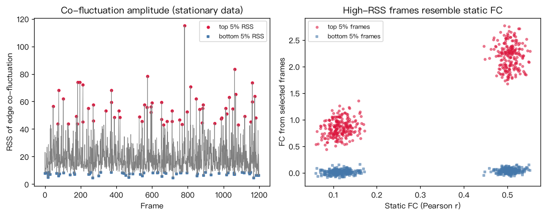
# 把每个脑区 z 标准化后，边 (i,j) 的边时间序列为逐点乘积 e_ij(t) = z_i(t) z_j(t)；
# 它在时间上的平均恰好等于皮尔逊相关（用总体标准差标准化时严格相等）。
# 每帧的共波动幅度用所有边的均方根（RSS）表示，取最高与最低 5% 的帧分别重建 FC，与整段 FC 比较。
# 模拟数据是一个“平稳”的多元高斯过程（真实 FC 恒定），用来说明：即使没有任何动态，
# 高 RSS 帧也会更像整体 FC（与 Ladwig 等 2022、Novelli & Razi 2022 的论证一致）。
import numpy as np

rng = np.random.default_rng(7)
N, T = 30, 1200
# 两个模块的平稳协方差（模拟数据，仅用于演示方法）
C = np.full((N, N), 0.1)
C[:15, :15] = C[15:, 15:] = 0.5
np.fill_diagonal(C, 1.0)
X = rng.multivariate_normal(np.zeros(N), C, size=T).T
Z = (X - X.mean(1, keepdims=True)) / X.std(1, keepdims=True)

iu = np.triu_indices(N, 1)
E = Z[iu[0]] * Z[iu[1]]                        # (边数, T) 边时间序列
r_static = np.corrcoef(X)[iu]
print("边时间序列的时间平均 与 皮尔逊 r 的最大差异 =", np.abs(E.mean(1) - r_static).max().round(12))

rss = np.sqrt((E ** 2).sum(0))
order = np.argsort(rss)
k = int(0.05 * T)
top, bottom = order[-k:], order[:k]
fc_top = E[:, top].mean(1)
fc_bot = E[:, bottom].mean(1)
print(f"最高 5% 帧重建的 FC 与整体 FC 的相关 = {np.corrcoef(fc_top, r_static)[0, 1]:.2f}")
print(f"最低 5% 帧重建的 FC 与整体 FC 的相关 = {np.corrcoef(fc_bot, r_static)[0, 1]:.2f}")
rand = rng.choice(T, k, replace=False)
print(f"随机 5% 帧重建的 FC 与整体 FC 的相关 = {np.corrcoef(E[:, rand].mean(1), r_static)[0, 1]:.2f}")

import matplotlib.pyplot as plt
fig, axes = plt.subplots(1, 2, figsize=(10, 4))
axes[0].plot(rss, color="gray", lw=0.6)
axes[0].scatter(top, rss[top], s=10, color="crimson", label="top 5% RSS")
axes[0].scatter(bottom, rss[bottom], s=10, color="#4477AA", marker="s", label="bottom 5% RSS")
axes[0].set(xlabel="Frame", ylabel="RSS of edge co-fluctuation", title="Co-fluctuation amplitude (stationary data)")
axes[0].legend(fontsize=8)
axes[1].scatter(r_static, fc_top, s=8, alpha=0.5, color="crimson", marker="o", label="top 5% frames")
axes[1].scatter(r_static, fc_bot, s=8, alpha=0.5, color="#4477AA", marker="s", label="bottom 5% frames")
axes[1].set(xlabel="Static FC (Pearson r)", ylabel="FC from selected frames", title="High-RSS frames resemble static FC")
axes[1].legend(fontsize=8)
plt.tight_layout(); plt.show()