Example10 / 11
小波相干:连接强度随时间和频率变化
用 Morlet 小波对两条信号做连续小波变换 W_x(s,t)、W_y(s,t), 小波相干 R²(s,t) = |S(W_x W_y*)|² / (S(|W_x|²) S(|W_y|²)),S 为时间方向的高斯平滑(尺度相关)。 模拟:两条信号共享一个周期 40 点的振荡,但只在前半段共享(模拟数据,仅用于演示方法)。 输出解读:周期 40 的相干在前半段接近 1、后半段明显下降;其他周期不随时间系统变化。 注意后半段及其他周期的相干仍有 0.4–0.7:平滑窗口有限时小波相干有正偏差,必须与替代数据比较而非与 0 比较。 实际分析还要剔除“影响锥”(cone of influence)内的边缘值,并用蒙特卡洛替代数据评估显著性。
Output输出图
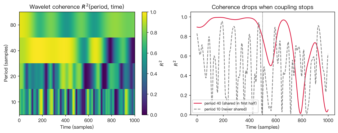
Output文字输出
周期  10:前半段平均相干 0.52,后半段 0.47
周期  20:前半段平均相干 0.50,后半段 0.41
周期  40:前半段平均相干 0.98,后半段 0.62
周期  80:前半段平均相干 0.71,后半段 0.72
Code代码
# 用 Morlet 小波对两条信号做连续小波变换 W_x(s,t)、W_y(s,t),
# 小波相干 R²(s,t) = |S(W_x W_y*)|² / (S(|W_x|²) S(|W_y|²)),S 为时间方向的高斯平滑(尺度相关)。
# 模拟:两条信号共享一个周期 40 点的振荡,但只在前半段共享(模拟数据,仅用于演示方法)。
# 输出解读:周期 40 的相干在前半段接近 1、后半段明显下降;其他周期不随时间系统变化。
# 注意后半段及其他周期的相干仍有 0.4–0.7:平滑窗口有限时小波相干有正偏差,必须与替代数据比较而非与 0 比较。
# 实际分析还要剔除“影响锥”(cone of influence)内的边缘值,并用蒙特卡洛替代数据评估显著性。
import numpy as np

rng = np.random.default_rng(8)
T = 1000
t = np.arange(T)
common = np.sin(2 * np.pi * t / 40)
x = common + rng.standard_normal(T)
y = np.where(t < T // 2, common, 0.0) + rng.standard_normal(T)   # 后半段不再含共同振荡

def morlet_cwt(sig, periods, w0=6.0):
    """FFT 实现的 Morlet 连续小波变换;periods 以采样点为单位。"""
    n = len(sig)
    f = np.fft.fftfreq(n)
    F = np.fft.fft(sig - sig.mean())
    out = np.zeros((len(periods), n), dtype=complex)
    for i, P in enumerate(periods):
        s = P * w0 / (2 * np.pi)                     # Morlet:周期 ≈ 2π s / w0
        psi_hat = np.pi ** -0.25 * np.exp(-0.5 * (s * 2 * np.pi * f - w0) ** 2) * (f > 0)
        out[i] = np.fft.ifft(F * psi_hat * np.sqrt(2 * np.pi * s))
    return out

def smooth_time(M, periods, w0=6.0):
    out = np.empty_like(M)
    for i, P in enumerate(periods):
        s = P * w0 / (2 * np.pi)
        k = np.exp(-0.5 * (np.arange(-3 * int(s) - 1, 3 * int(s) + 2) / s) ** 2)
        k /= k.sum()
        out[i] = np.convolve(M[i], k, mode="same")
    return out

periods = np.array([10, 20, 40, 80])
Wx, Wy = morlet_cwt(x, periods), morlet_cwt(y, periods)
num = np.abs(smooth_time(Wx * np.conj(Wy), periods)) ** 2
den = smooth_time(np.abs(Wx) ** 2, periods).real * smooth_time(np.abs(Wy) ** 2, periods).real
R2 = num / den
first, second = slice(100, 400), slice(600, 900)    # 避开边缘
for P, r in zip(periods, R2):
    print(f"周期 {P:3d}:前半段平均相干 {r[first].mean():.2f},后半段 {r[second].mean():.2f}")

import matplotlib.pyplot as plt
fig, axes = plt.subplots(1, 2, figsize=(10, 4))
im = axes[0].imshow(R2, aspect="auto", cmap="viridis", vmin=0, vmax=1, origin="lower", interpolation="nearest",
                    extent=[0, T, -0.5, len(periods) - 0.5])
axes[0].set(yticks=range(len(periods)), yticklabels=periods, xlabel="Time (samples)", ylabel="Period (samples)",
            title="Wavelet coherence $R^2$(period, time)")
fig.colorbar(im, ax=axes[0], label="$R^2$")
axes[1].plot(t, R2[2], "-", color="crimson", label="period 40 (shared in first half)")
axes[1].plot(t, R2[0], "--", color="gray", label="period 10 (never shared)")
axes[1].axvline(T // 2, color="k", ls=":", lw=1)
axes[1].set(xlabel="Time (samples)", ylabel="$R^2$", ylim=(0, 1.05), title="Coherence drops when coupling stops")
axes[1].legend(fontsize=8, loc="lower left")
plt.tight_layout(); plt.show()Run在浏览器中运行
首次加载 Python 环境约需 20–40 秒;可以修改参数后重新运行。