Example02 / 09
拓扑重叠矩阵(TOM)与层次聚类划分模块
用无标度拟合准则选出的 β 构建邻接矩阵,计算 TOM_ij = (l_ij + a_ij) / (min(k_i, k_j) + 1 − a_ij),l = A·A; 以 1 − TOM 为距离做平均连锁层次聚类,在高度 0.93 处切树,少于 10 个基因的小簇记为 0 (相当于 WGCNA 中未归类的灰色基因),再与真实模块标签做列联表。 输出解读:4 个真实模块基本被完整找回,噪声基因大多落在 0 类;热图中模块沿对角线呈块状。 切树高度与最小模块大小会改变结果(例如改成 0.98 与 5),真实分析中应报告这些参数并检验稳定性。
Output输出图
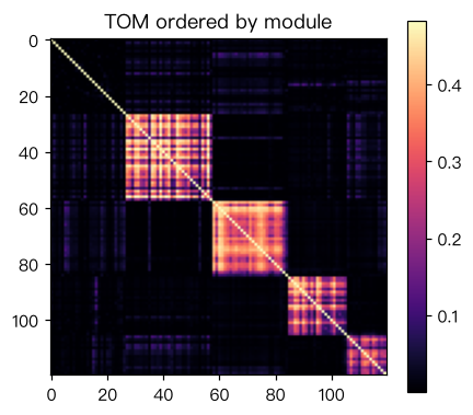
Output文字输出
beta = 3;找到 4 个模块;列联表(行 = 真实标签 0..4,列 = 聚类 0..4,0 为未归类):
0 [27, 1, 2, 0, 0]
1 [0, 30, 0, 0, 0]
2 [0, 0, 25, 0, 0]
3 [0, 0, 0, 20, 0]
4 [0, 0, 0, 1, 14]
Code代码
# 用无标度拟合准则选出的 β 构建邻接矩阵,计算 TOM_ij = (l_ij + a_ij) / (min(k_i, k_j) + 1 − a_ij),l = A·A;
# 以 1 − TOM 为距离做平均连锁层次聚类,在高度 0.93 处切树,少于 10 个基因的小簇记为 0
# (相当于 WGCNA 中未归类的灰色基因),再与真实模块标签做列联表。
# 输出解读:4 个真实模块基本被完整找回,噪声基因大多落在 0 类;热图中模块沿对角线呈块状。
# 切树高度与最小模块大小会改变结果(例如改成 0.98 与 5),真实分析中应报告这些参数并检验稳定性。
import numpy as np
from scipy import stats
from scipy.cluster.hierarchy import linkage, fcluster
from scipy.spatial.distance import squareform
import matplotlib.pyplot as plt

def simulate(seed=13):
    rng = np.random.default_rng(seed)
    n, sizes = 60, [30, 25, 20, 15]
    trait = rng.normal(size=n)
    factors = [0.8 * trait + 0.6 * rng.normal(size=n)] + [rng.normal(size=n) for _ in sizes[1:]]
    X, labels, load = [], [], []
    for m, (s, f) in enumerate(zip(sizes, factors)):
        for l in rng.uniform(0.5, 0.95, size=s):
            X.append(l * f + np.sqrt(1 - l**2) * rng.normal(size=n))
            labels.append(m + 1); load.append(l)
    for _ in range(30):
        X.append(rng.normal(size=n)); labels.append(0); load.append(0.0)
    return np.array(X).T, np.array(labels), np.array(load), trait

def scale_free_fit(A, nbins=10):
    k = A.sum(axis=1) - 1.0
    cnt, edges = np.histogram(k, bins=nbins)
    mid = (edges[:-1] + edges[1:]) / 2
    ok = cnt > 0
    res = stats.linregress(np.log10(mid[ok]), np.log10(cnt[ok] / cnt.sum()))
    return -np.sign(res.slope) * res.rvalue**2

def tom(A):
    """TOM_ij = (l_ij + a_ij) / (min(k_i, k_j) + 1 − a_ij),l = A @ A;A 的对角线须为 0。"""
    k = A.sum(axis=1)
    T = (A @ A + A) / (np.minimum.outer(k, k) + 1 - A)
    np.fill_diagonal(T, 1.0)
    return T

def cut_modules(Z, height=0.93, min_size=10):
    """按高度切树;小于 min_size 的簇记为 0;其余按大小从大到小编号 1, 2, ..."""
    c = fcluster(Z, t=height, criterion="distance")
    ids, counts = np.unique(c, return_counts=True)
    big = [i for i, n in sorted(zip(ids, counts), key=lambda x: -x[1]) if n >= min_size]
    return np.array([big.index(x) + 1 if x in big else 0 for x in c])

X, true_lab, true_load, trait = simulate()
R = np.corrcoef(X.T)
beta = next(b for b in range(1, 13) if scale_free_fit(np.abs(R) ** b) >= 0.85)
A = np.abs(R) ** beta
np.fill_diagonal(A, 0.0)

T = tom(A)
dist = 1.0 - T
np.fill_diagonal(dist, 0.0)
Z = linkage(squareform(dist, checks=False), method="average")
clusters = cut_modules(Z)
K = clusters.max()
print(f"beta = {beta};找到 {K} 个模块;列联表(行 = 真实标签 0..4,列 = 聚类 0..{K},0 为未归类):")
for t in range(5):
    print(t, [int(np.sum((true_lab == t) & (clusters == c))) for c in range(K + 1)])

order = np.argsort(clusters, kind="stable")
plt.figure(figsize=(4.5, 4))
plt.imshow(T[np.ix_(order, order)], cmap="magma", vmax=np.percentile(T, 99))
plt.title("TOM ordered by module"); plt.colorbar(); plt.show()Run在浏览器中运行
首次加载 Python 环境约需 20–40 秒;可以修改参数后重新运行。