互作组补全——共同邻居（L2）与长度为 3 的路径（L3）链路预测

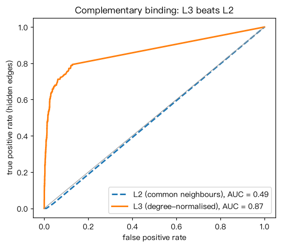
# Kovács 等（2019）指出：蛋白往往通过互补界面结合，A 与 B 相互作用，并不意味着 A 与 B 的伙伴相似；
# 但若 A 与 B 的某个伙伴相似（共享伙伴），则 A 更可能与 B 结合，因此应数长度为 3 的路径（L3）。
# 这里用“界面类型互补”生成模拟网络：每个蛋白有一个类型，类型 t 只与互补类型 partner[t] 结合。
# 隐藏 10% 的边，比较 L2（共同邻居数）与度归一化 L3 打分对隐藏边的排序 AUC。
# 输出解读：在互补结合主导的网络中，L3 的 AUC 明显高于 L2；在社交网络式的“相似者相连”网络中结论可能相反。
import numpy as np
import networkx as nx

rng = np.random.default_rng(0)
n, n_types = 600, 30                                  # 模拟数据，仅用于演示方法
types = rng.integers(n_types, size=n)
partner = {t: (t + n_types // 2) % n_types for t in range(n_types)}   # 互补类型配对
G = nx.Graph(); G.add_nodes_from(range(n))
for i in range(n):
    for j in range(i + 1, n):
        p = 0.25 if partner[types[i]] == types[j] else 0.002
        if rng.random() < p:
            G.add_edge(i, j)

edges = list(G.edges())
idx = rng.permutation(len(edges))
hidden = [edges[k] for k in idx[: len(edges) // 10]]
G_obs = G.copy(); G_obs.remove_edges_from(hidden)
A = nx.to_numpy_array(G_obs, nodelist=range(n))
k = A.sum(1); k[k == 0] = 1
L2 = A @ A
Dm = np.diag(1 / np.sqrt(k))
L3 = A @ Dm @ A @ Dm @ A                               # p_XY = Σ a_XU a_UV a_VY / sqrt(k_U k_V)

def auc(score, pos, neg):
    s_pos = np.array([score[i, j] for i, j in pos]); s_neg = np.array([score[i, j] for i, j in neg])
    # AUC = P(正例得分 > 负例得分)，平局记 0.5
    gt = (s_pos[:, None] > s_neg[None, :]).mean(); eq = (s_pos[:, None] == s_neg[None, :]).mean()
    return gt + 0.5 * eq

neg = []
while len(neg) < 3000:
    i, j = rng.integers(n, size=2)
    if i != j and not G.has_edge(i, j):
        neg.append((i, j))
print(f"节点 {n}，边 {G.number_of_edges()}，隐藏 {len(hidden)} 条")
print(f"AUC：L2（共同邻居）= {auc(L2, hidden, neg):.3f}，L3（度归一化）= {auc(L3, hidden, neg):.3f}")

import matplotlib.pyplot as plt
def roc(score, pos, neg):
    """在每个不同的得分阈值处计算 (FPR, TPR)；并列得分之间线性连接，与平局记 0.5 的 AUC 一致。"""
    sp_ = np.sort([score[i, j] for i, j in pos]); sn_ = np.sort([score[i, j] for i, j in neg])
    thr = np.r_[np.inf, np.unique(np.r_[sp_, sn_])[::-1]]
    return 1 - np.searchsorted(sn_, thr) / len(sn_), 1 - np.searchsorted(sp_, thr) / len(sp_)
fig, ax = plt.subplots(figsize=(5.2, 4.6))
for S, lab, ls in [(L2, "L2 (common neighbours)", "--"), (L3, "L3 (degree-normalised)", "-")]:
    fpr, tpr = roc(S, hidden, neg)
    ax.plot(fpr, tpr, ls, lw=2, label=f"{lab}, AUC = {auc(S, hidden, neg):.2f}")
ax.plot([0, 1], [0, 1], color="0.6", lw=0.8)
ax.set_xlabel("false positive rate"); ax.set_ylabel("true positive rate (hidden edges)")
ax.set_title("Complementary binding: L3 beats L2"); ax.legend(loc="lower right")
plt.tight_layout(); plt.show()