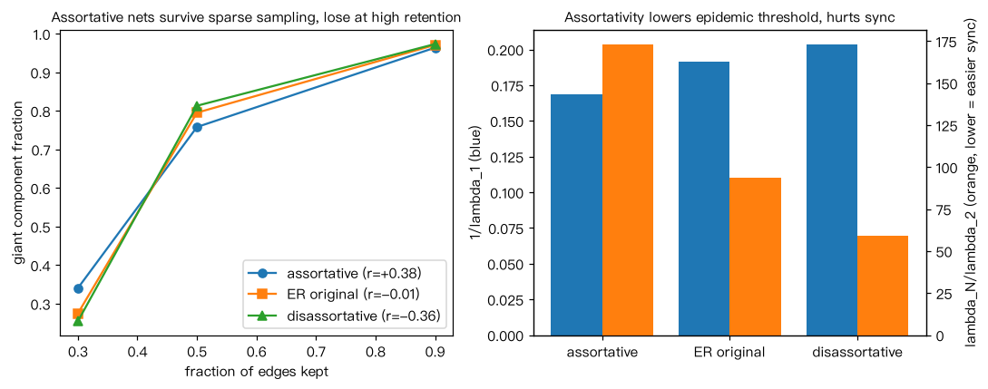
度相关如何改变巨连通分支、传播阈值与可同步性

# 从同一张 ER 随机图（N=2000, <k>=4）出发，用 Xulvi-Brunet–Sokolov 重连（p=0.5）得到同配与异配版本。
# 比较：(1) 随机删边（键渗流）后巨连通分支占比；(2) 邻接矩阵最大特征值 lambda_1，
#   SIS 模型的淬火平均场阈值约为 1/lambda_1；(3) 拉普拉斯特征值比 lambda_N/lambda_2（越小越易同步）。
# 解读：同配使 lambda_1 增大（高度节点聚在一起形成“储库”，阈值降低）、低保留率下巨分支更易存活，
# 但高保留率下巨分支更小；同配同时使 lambda_N/lambda_2 增大，可同步性变差。
import numpy as np
import networkx as nx
from scipy.sparse.linalg import eigsh
from scipy.sparse.csgraph import laplacian


def xbs_rewire(G, n_swaps, mode, p, seed):
    rng = np.random.default_rng(seed)
    G = G.copy(); dg = dict(G.degree()); edges = list(G.edges()); done = 0
    while done < n_swaps:
        i, j = rng.choice(len(edges), 2, replace=False)
        (a, b), (c, d) = edges[i], edges[j]
        nodes = [a, b, c, d]
        if len(set(nodes)) < 4:
            continue
        if rng.random() < p:
            s = sorted(nodes, key=lambda x: dg[x], reverse=True)
            new = [(s[0], s[1]), (s[2], s[3])] if mode == "assortative" else [(s[0], s[3]), (s[1], s[2])]
        else:
            rng.shuffle(nodes)
            new = [(nodes[0], nodes[1]), (nodes[2], nodes[3])]
        if any(G.has_edge(*e) for e in new):
            continue
        G.remove_edges_from([(a, b), (c, d)]); G.add_edges_from(new)
        edges[i], edges[j] = new; done += 1
    return G


def giant_after_bond_percolation(G, keep, n_rep=10, seed=0):
    rng = np.random.default_rng(seed)
    edges = list(G.edges())
    out = []
    for _ in range(n_rep):
        H = nx.Graph()
        H.add_nodes_from(G)
        H.add_edges_from([e for e in edges if rng.random() < keep])
        out.append(max(len(c) for c in nx.connected_components(H)) / G.number_of_nodes())
    return np.mean(out)


G0 = nx.gnm_random_graph(2000, 4000, seed=1)
M = G0.number_of_edges()
nets = {
    "同配 (p=0.5)": xbs_rewire(G0, 3 * M, "assortative", 0.5, 1),
    "ER 原始": G0,
    "异配 (p=0.5)": xbs_rewire(G0, 3 * M, "disassortative", 0.5, 2),
}
print("保留边比例:            0.30    0.50    0.90")
summ = []                                    # 保存结果用于作图
for name, G in nets.items():
    A = nx.to_scipy_sparse_array(G, dtype=float, format="csr")
    lam1 = eigsh(A, k=1, which="LA")[0][0]
    S = [giant_after_bond_percolation(G, q, seed=3) for q in (0.3, 0.5, 0.9)]
    Gc = G.subgraph(max(nx.connected_components(G), key=len))
    L = laplacian(nx.to_numpy_array(Gc))
    ev = np.sort(np.linalg.eigvalsh(L))
    print(f"{name:12s} r={nx.degree_assortativity_coefficient(G):+.2f}  巨分支占比 "
          f"{S[0]:.3f}  {S[1]:.3f}  {S[2]:.3f} | lambda_1={lam1:.2f} (SIS 阈值≈{1/lam1:.3f}) "
          f"| lambda_N/lambda_2={ev[-1]/ev[1]:.1f}")
    summ.append((nx.degree_assortativity_coefficient(G), S, lam1, ev[-1] / ev[1]))

# 作图：键渗流后的巨分支占比，以及 SIS 阈值与同步性指标
import matplotlib.pyplot as plt
fig, ax = plt.subplots(1, 2, figsize=(10, 4))
labs = ["assortative", "ER original", "disassortative"]
for (r, S, lam1, ratio), lab, mk in zip(summ, labs, ["o", "s", "^"]):
    ax[0].plot([0.3, 0.5, 0.9], S, marker=mk, label=f"{lab} (r={r:+.2f})")
ax[0].set_xlabel("fraction of edges kept"); ax[0].set_ylabel("giant component fraction"); ax[0].legend()
ax[0].set_title("Assortative nets survive sparse sampling, lose at high retention", fontsize=10)
x = np.arange(3)
ax[1].bar(x - 0.2, [1 / s[2] for s in summ], 0.4, label="SIS threshold 1/lambda_1")
ax2 = ax[1].twinx()
ax2.bar(x + 0.2, [s[3] for s in summ], 0.4, color="C1", label="lambda_N/lambda_2")
ax[1].set_xticks(x); ax[1].set_xticklabels(labs); ax[1].set_ylabel("1/lambda_1 (blue)")
ax2.set_ylabel("lambda_N/lambda_2 (orange, lower = easier sync)")
ax[1].set_title("Assortativity lowers epidemic threshold, hurts sync", fontsize=10)
plt.tight_layout(); plt.show()