k-核分解——手写剥离算法并与 NetworkX 对照，比较核数与度

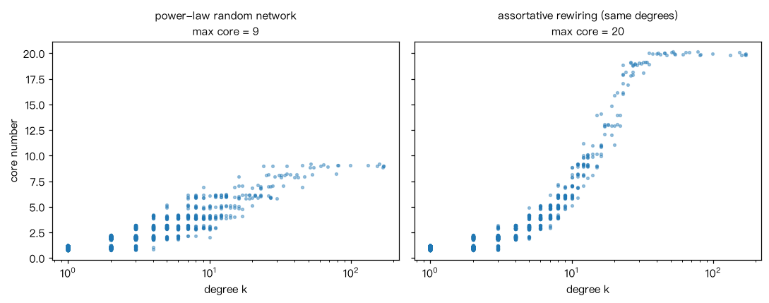
# 实现 Batagelj–Zaversnik 的“按当前度从小到大剥离”思想（这里用简单的最小堆，复杂度 O(M log N)），
# 与 nx.core_number 对照；再在一个幂律随机网络与一个“度相同但枢纽之间互连更多”的网络上比较：
# （不用 BA 网络：BA 网络每个新节点恰好带 m 条边，整张图就是一个 m-核，壳层结构是平凡的。）
# 最内核大小、最内核内部密度，以及核数与度的 Spearman 相关。
# 解读：核数度量的是“嵌在多稠密的子图里”，与度高度相关但不等同；度相同的节点可以处在很不同的壳层。
import heapq
import numpy as np
import networkx as nx
from scipy.stats import spearmanr


def core_numbers(G):
    deg = dict(G.degree())
    heap = [(d, v) for v, d in deg.items()]
    heapq.heapify(heap)
    removed, core, k = set(), {}, 0
    while heap:
        d, v = heapq.heappop(heap)
        if v in removed or d != deg[v]:
            continue                      # 过期的堆元素
        k = max(k, d)                     # 当前壳层编号只增不减
        core[v] = k
        removed.add(v)
        for u in G[v]:
            if u not in removed:
                deg[u] -= 1
                heapq.heappush(heap, (deg[u], u))
    return core


rng = np.random.default_rng(2)
deg_seq = np.minimum(np.floor((1 - rng.random(3000)) ** (-1 / 1.3)).astype(int), 200)   # 幂律，gamma≈2.3，k_min=1
if deg_seq.sum() % 2:
    deg_seq[0] += 1
G = nx.Graph(nx.configuration_model(deg_seq.tolist(), seed=2))
G.remove_edges_from(nx.selfloop_edges(G))
core = core_numbers(G)
print("手写剥离算法与 nx.core_number 一致:", core == nx.core_number(G))

# 一个度序列相同、但用同配重连让高度节点彼此相连的网络
def assort_rewire(G, n_swaps, seed):
    rng = np.random.default_rng(seed)
    G = G.copy(); dg = dict(G.degree()); edges = list(G.edges()); done = 0
    while done < n_swaps:
        i, j = rng.choice(len(edges), 2, replace=False)
        (a, b), (c, d) = edges[i], edges[j]
        if len({a, b, c, d}) < 4:
            continue
        s = sorted([a, b, c, d], key=lambda x: dg[x], reverse=True)
        new = [(s[0], s[1]), (s[2], s[3])]
        if any(G.has_edge(*e) for e in new):
            continue
        G.remove_edges_from([(a, b), (c, d)]); G.add_edges_from(new)
        edges[i], edges[j] = new; done += 1
    return G


Ga = assort_rewire(G, G.number_of_edges(), seed=3)
for name, H in [("幂律随机网络", G), ("同配重连（度序列相同）", Ga)]:
    cn = nx.core_number(H)
    kmax = max(cn.values())
    inner = [v for v in H if cn[v] == kmax]
    sub = H.subgraph(inner)
    deg = dict(H.degree())
    rho = spearmanr([deg[v] for v in H], [cn[v] for v in H])[0]
    print(f"{name}: r = {nx.degree_assortativity_coefficient(H):+.2f}, 最大核数 k_s^max = {kmax}, "
          f"最内核节点数 = {len(inner)}, 最内核内部密度 = {nx.density(sub):.2f}, 核数与度的 Spearman = {rho:.2f}")

# 同一度的节点可以位于不同壳层
deg = dict(G.degree())
k_ex = 6
shells = sorted({core[v] for v in G if deg[v] == k_ex})
print(f"幂律随机网络中度为 {k_ex} 的节点分布在这些壳层: {shells}")

# 作图：度 vs 核数（加少量抖动以显示重叠点）
import matplotlib.pyplot as plt
fig, ax = plt.subplots(1, 2, figsize=(10, 4), sharey=True)
jit = np.random.default_rng(0)
for a, H, ttl in [(ax[0], G, "power-law random network"), (ax[1], Ga, "assortative rewiring (same degrees)")]:
    cn = nx.core_number(H)
    x = np.array([H.degree(v) for v in H]); y = np.array([cn[v] for v in H], float)
    a.scatter(x, y + jit.uniform(-0.2, 0.2, len(y)), s=6, alpha=0.4)
    a.set_xscale("log"); a.set_xlabel("degree k"); a.set_title(f"{ttl}\nmax core = {int(y.max())}", fontsize=10)
ax[0].set_ylabel("core number")
plt.tight_layout(); plt.show()