Example01 / 11
全连接 Kuramoto 模型的同步相变
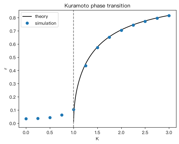
固有频率取洛伦兹分布(半宽 gamma=0.5),理论临界耦合 K_c = 2*gamma = 1, 超过临界值后 r = sqrt(1 - K_c/K)。simulate 用平均场形式做欧拉积分, 扫描 K = 0, 0.25, …, 3,记录每个 K 的稳态 r(后一半时间的平均),与理论曲线画在一张图上。 解读:K<1 时 r 很小(只剩约 1/sqrt(N) 的有限尺度基线),K>1 后 r 迅速上升并贴近理论值。
Output输出图
Output文字输出
K: [0.0, 0.25, 0.5, 0.75, 1.0, 1.25, 1.5, 1.75, 2.0, 2.25, 2.5, 2.75, 3.0]
r: [0.03, 0.04, 0.04, 0.06, 0.1, 0.44, 0.57, 0.65, 0.7, 0.74, 0.77, 0.8, 0.81]
Code代码
# 固有频率取洛伦兹分布(半宽 gamma=0.5),理论临界耦合 K_c = 2*gamma = 1,
# 超过临界值后 r = sqrt(1 - K_c/K)。simulate 用平均场形式做欧拉积分,
# 扫描 K = 0, 0.25, ..., 3,记录每个 K 的稳态 r(后一半时间的平均),与理论曲线画在一张图上。
# 解读:K<1 时 r 很小(只剩约 1/sqrt(N) 的有限尺度基线),K>1 后 r 迅速上升并贴近理论值。
import numpy as np
import matplotlib.pyplot as plt

N, gamma = 500, 0.5
# 用分位数取样代替随机抽样,减少有限尺度涨落(洛伦兹分布的反函数为 gamma*tan)
omega = gamma * np.tan(np.pi * (np.arange(1, N + 1) / (N + 1) - 0.5))

def simulate(K, omega, T=60.0, dt=0.05, seed=0):
    rng = np.random.default_rng(seed)
    theta = rng.uniform(0, 2 * np.pi, omega.size)
    rs = []
    for _ in range(int(T / dt)):
        z = np.exp(1j * theta).mean()            # 序参量 r*e^{i psi}
        theta = theta + dt * (omega + K * np.imag(z * np.exp(-1j * theta)))
        rs.append(abs(z))
    rs = np.array(rs)
    return rs[len(rs) // 2:].mean()

Ks = np.arange(0, 3.01, 0.25)
r_sim = np.array([simulate(K, omega) for K in Ks])
print("K:", np.round(Ks, 2).tolist())
print("r:", np.round(r_sim, 2).tolist())

K_th = np.linspace(1.0001, 3, 200)
plt.plot(K_th, np.sqrt(1 - 2 * gamma / K_th), "k-", label="theory")
plt.plot(Ks, r_sim, "o", label="simulation")
plt.axvline(2 * gamma, ls="--", c="gray")
plt.xlabel("K"); plt.ylabel("r"); plt.legend(); plt.title("Kuramoto phase transition")
plt.show()Run在浏览器中运行
首次加载 Python 环境约需 20–40 秒;可以修改参数后重新运行。