Example11 / 11
PLV、PLI、wPLI、相干与虚部相干:容积传导的影响
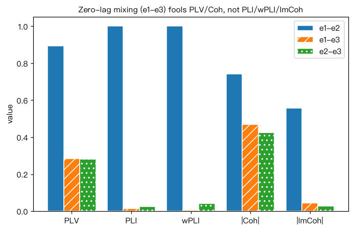
构造两个真实源:s1 为 10 Hz 振荡(带相位噪声),s2 是 s1 延迟 20 ms 的版本加独立噪声, 即两源之间存在“滞后的真实耦合”。另有一个无关源 s3。电极信号是源的线性混合(容积传导): e1 = s1 + 0.5 s3, e2 = s2 + 0.5 s3, e3 = s3 + 噪声(e3 与 e1/e2 只通过 s3 的混合“相关”)。 对每对电极在 8–12 Hz 带通后计算:PLV、PLI、wPLI、幅度相干 |Coh| 与虚部相干 |ImCoh|, 并用时间平移替代数据(circular shift)得到 PLV 的 95% 零分布分位数。 解读:e1–e3 只有零滞后的混合,PLV 与 |Coh| 显著偏高,而 PLI、wPLI、ImCoh 接近 0; e1–e2 存在滞后耦合,所有指标都高。
Output输出图
Output文字输出
e1-e2  PLV=0.89 (替代95%=0.25)  PLI=1.00  wPLI=1.00  |Coh|=0.74  |ImCoh|=0.56
e1-e3  PLV=0.29 (替代95%=0.10)  PLI=0.01  wPLI=0.01  |Coh|=0.47  |ImCoh|=0.04
e2-e3  PLV=0.28 (替代95%=0.11)  PLI=0.02  wPLI=0.04  |Coh|=0.42  |ImCoh|=0.03
Code代码
# 构造两个真实源:s1 为 10 Hz 振荡(带相位噪声),s2 是 s1 延迟 20 ms 的版本加独立噪声,
# 即两源之间存在“滞后的真实耦合”。另有一个无关源 s3。电极信号是源的线性混合(容积传导):
#   e1 = s1 + 0.5 s3,  e2 = s2 + 0.5 s3,  e3 = s3 + 噪声(e3 与 e1/e2 只通过 s3 的混合“相关”)。
# 对每对电极在 8–12 Hz 带通后计算:PLV、PLI、wPLI、幅度相干 |Coh| 与虚部相干 |ImCoh|,
# 并用时间平移替代数据(circular shift)得到 PLV 的 95% 零分布分位数。
# 解读:e1–e3 只有零滞后的混合,PLV 与 |Coh| 显著偏高,而 PLI、wPLI、ImCoh 接近 0;
#       e1–e2 存在滞后耦合,所有指标都高。
import numpy as np
from scipy.signal import butter, filtfilt, hilbert, csd, welch

fs, T = 250, 120
t = np.arange(int(fs * T)) / fs
rng = np.random.default_rng(0)
phase = 2 * np.pi * 10 * t + np.cumsum(rng.standard_normal(t.size)) * 0.05
s1 = np.cos(phase) + 0.5 * rng.standard_normal(t.size)
lag = int(0.020 * fs)
s2 = np.roll(np.cos(phase), lag) + 0.5 * rng.standard_normal(t.size)
s3 = np.cos(2 * np.pi * 10.5 * t + np.cumsum(rng.standard_normal(t.size)) * 0.05) + 0.5 * rng.standard_normal(t.size)
e = {"e1": s1 + 0.5 * s3, "e2": s2 + 0.5 * s3, "e3": s3 + 0.5 * rng.standard_normal(t.size)}

bb, aa = butter(4, [8, 12], btype="band", fs=fs)
an = {k: hilbert(filtfilt(bb, aa, v)) for k, v in e.items()}

def metrics(x, y):
    S = x * np.conj(y)                               # 瞬时交叉谱
    dphi = np.angle(S)
    plv = abs(np.mean(np.exp(1j * dphi)))
    pli = abs(np.mean(np.sign(np.sin(dphi))))
    wpli = abs(np.mean(S.imag)) / np.mean(np.abs(S.imag))
    return plv, pli, wpli

def coherence(x, y, band=(8, 12)):
    f, Sxy = csd(x, y, fs=fs, nperseg=fs * 2)
    _, Sxx = welch(x, fs=fs, nperseg=fs * 2); _, Syy = welch(y, fs=fs, nperseg=fs * 2)
    m = (f >= band[0]) & (f <= band[1])
    coh = Sxy[m] / np.sqrt(Sxx[m] * Syy[m])
    return abs(coh).mean(), abs(coh.imag).mean()

table = {}
for p, q in [("e1", "e2"), ("e1", "e3"), ("e2", "e3")]:
    plv, pli, wpli = metrics(an[p], an[q])
    ch, ich = coherence(e[p], e[q])
    null = [abs(np.mean(np.exp(1j * np.angle(an[p] * np.conj(np.roll(an[q], s))))))
            for s in rng.integers(fs * 5, t.size - fs * 5, 200)]
    table[p + "-" + q] = [plv, pli, wpli, ch, ich]
    print("%s-%s  PLV=%.2f (替代95%%=%.2f)  PLI=%.2f  wPLI=%.2f  |Coh|=%.2f  |ImCoh|=%.2f"
          % (p, q, plv, np.quantile(null, 0.95), pli, wpli, ch, ich))

import matplotlib.pyplot as plt
fig, ax = plt.subplots(figsize=(6.4, 4.2))
metric_names = ["PLV", "PLI", "wPLI", "|Coh|", "|ImCoh|"]
x = np.arange(len(metric_names))
for j, ((pair, v), hatch) in enumerate(zip(table.items(), ["", "//", ".."])):
    ax.bar(x + (j - 1) * 0.27, v, 0.27, hatch=hatch, label=pair, edgecolor="white")
ax.set_xticks(x, metric_names); ax.set_ylabel("value"); ax.set_ylim(0, 1.05); ax.legend()
ax.set_title("Zero-lag mixing (e1-e3) fools PLV/Coh, not PLI/wPLI/ImCoh", fontsize=10)
plt.tight_layout(); plt.show()Run在浏览器中运行
首次加载 Python 环境约需 20–40 秒;可以修改参数后重新运行。