Example09 / 11
噪声与时滞对 Kuramoto 同步的影响
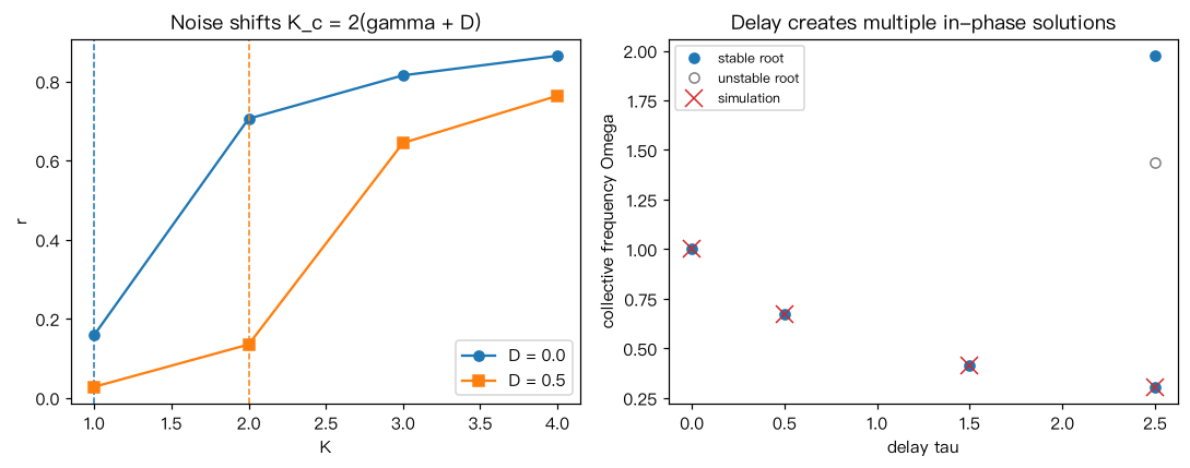
- 噪声:全连接 Kuramoto + 白噪声 d theta = [omega + K r sin(psi-theta)] dt + sqrt(2D) dW, omega 取洛伦兹分布(gamma=0.5)。理论 K_c = 2(gamma + D)。用 Euler–Maruyama 积分, 比较 D=0 与 D=0.5 时 r(K) 的起点。
- 时滞:两个相同振荡器 omega=1、耦合 K=1、时滞 tau,完全同步时集体频率满足 Omega = omega - K sin(Omegatau);同相态稳定需 K cos(Omegatau) > 0。tau 较大时有多个解(多稳态), 模拟落在哪一个取决于初始历史。
Output输出图
Output文字输出
D=0.0 理论 K_c=1.0  r(K=1,2,3,4) = [0.16, 0.71, 0.82, 0.86]
D=0.5 理论 K_c=2.0  r(K=1,2,3,4) = [0.03, 0.14, 0.64, 0.76]
tau=0.0  同相解 Omega: [1.0]  其中稳定: [1.0]
         模拟(初值接近、历史取常数)得到 Omega=1.000,末态相位差=-0.00
tau=0.5  同相解 Omega: [0.671]  其中稳定: [0.671]
         模拟(初值接近、历史取常数)得到 Omega=0.671,末态相位差=0.00
tau=1.5  同相解 Omega: [0.416]  其中稳定: [0.416]
         模拟(初值接近、历史取常数)得到 Omega=0.416,末态相位差=0.00
tau=2.5  同相解 Omega: [0.307, 1.438, 1.975]  其中稳定: [0.307, 1.975]
模拟(初值接近、历史取常数)得到 Omega=0.307,末态相位差=0.00Code代码
# (1) 噪声:全连接 Kuramoto + 白噪声 d theta = [omega + K r sin(psi-theta)] dt + sqrt(2D) dW,
#     omega 取洛伦兹分布(gamma=0.5)。理论 K_c = 2(gamma + D)。用 Euler–Maruyama 积分,
#     比较 D=0 与 D=0.5 时 r(K) 的起点。
# (2) 时滞:两个相同振荡器 omega=1、耦合 K=1、时滞 tau,完全同步时集体频率满足
#     Omega = omega - K sin(Omega*tau);同相态稳定需 K cos(Omega*tau) > 0。tau 较大时有多个解(多稳态),
#     模拟落在哪一个取决于初始历史。
import numpy as np
from scipy.optimize import brentq

N, gamma = 2000, 0.5
omega = gamma * np.tan(np.pi * (np.arange(1, N + 1) / (N + 1) - 0.5))
def r_noise(K, D, T=60.0, dt=0.02, seed=0):
    rng = np.random.default_rng(seed)
    th = rng.uniform(0, 2 * np.pi, N); rs = []
    for n in range(int(T / dt)):
        z = np.exp(1j * th).mean()
        th = th + dt * (omega + K * np.imag(z * np.exp(-1j * th))) + np.sqrt(2 * D * dt) * rng.standard_normal(N)
        if n > int(T / dt) // 2:
            rs.append(abs(z))
    return np.mean(rs)
r_by_D = {}
for D in [0.0, 0.5]:
    Ks = [1.0, 2.0, 3.0, 4.0]
    r_by_D[D] = [r_noise(K, D) for K in Ks]
    print("D=%.1f 理论 K_c=%.1f  r(K=1,2,3,4) =" % (D, 2 * (gamma + D)),
          np.round(r_by_D[D], 2).tolist())

w, K = 1.0, 1.0
delay_res = []
for tau in [0.0, 0.5, 1.5, 2.5]:
    g = lambda O: O - w + K * np.sin(O * tau)        # 所有解都落在 [w-K, w+K]
    grid = np.linspace(w - K, w + K, 2001)
    roots = [brentq(g, x0, x1) for x0, x1 in zip(grid[:-1], grid[1:]) if g(x0) * g(x1) < 0]
    roots = roots or [w]
    stable = [O for O in roots if K * np.cos(O * tau) > 0]
    print("tau=%.1f  同相解 Omega:" % tau, np.round(roots, 3).tolist(), " 其中稳定:", np.round(stable, 3).tolist())
    # 模拟:两个振荡器,初始相位接近,用历史缓冲实现时滞
    dt = 0.001; d = int(round(tau / dt)); steps = 60000
    th = np.zeros((steps + 1, 2)); th[0] = [0.0, 0.1]
    for n in range(steps):
        past = th[max(n - d, 0)]
        th[n + 1, 0] = th[n, 0] + dt * (w + K * np.sin(past[1] - th[n, 0]))
        th[n + 1, 1] = th[n, 1] + dt * (w + K * np.sin(past[0] - th[n, 1]))
    Om_sim = (th[-1, 0] - th[-20001, 0]) / (20000 * dt)
    print("         模拟(初值接近、历史取常数)得到 Omega=%.3f,末态相位差=%.2f"
          % (Om_sim, np.angle(np.exp(1j * (th[-1, 0] - th[-1, 1])))))
    delay_res.append((tau, roots, stable, Om_sim))

import matplotlib.pyplot as plt
fig, (ax1, ax2) = plt.subplots(1, 2, figsize=(10, 4))
for (D, rs), mk in zip(r_by_D.items(), ["o", "s"]):
    l, = ax1.plot(Ks, rs, marker=mk, ls="-", label="D = %.1f" % D)
    ax1.axvline(2 * (gamma + D), ls="--", c=l.get_color(), lw=1)
ax1.set_xlabel("K"); ax1.set_ylabel("r"); ax1.legend(); ax1.set_title("Noise shifts K_c = 2(gamma + D)")
for i, (tau, roots, stable, Om) in enumerate(delay_res):
    unst = [O for O in roots if O not in stable]
    ax2.plot([tau] * len(stable), stable, "o", c="tab:blue", label="stable root" if i == 0 else None)
    ax2.plot([tau] * len(unst), unst, "o", mfc="none", c="0.5", label="unstable root" if i == 0 else None)
    ax2.plot(tau, Om, "x", c="tab:red", ms=10, label="simulation" if i == 0 else None)
ax2.set_xlabel("delay tau"); ax2.set_ylabel("collective frequency Omega"); ax2.legend(fontsize=8)
ax2.set_title("Delay creates multiple in-phase solutions")
plt.tight_layout(); plt.show()Run在浏览器中运行
首次加载 Python 环境约需 20–40 秒;可以修改参数后重新运行。