比例阈值与密度匹配——整体连接强度差异如何“制造”拓扑差异

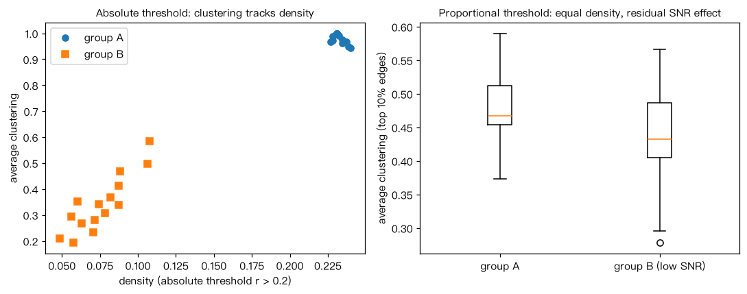
# 两组模拟被试拥有完全相同的模块结构，只是 B 组的系统内信号整体更弱（例如头动更大或信噪比更低）。
# 比较三种做法下的组间差异：(1) 绝对阈值；(2) 比例阈值（各被试保留最强的前 10% 边）；
# (3) 在 10%–30% 密度范围上积分（曲线下面积），并把聚集系数除以同度序列随机网络的值做归一化。
# 依次模拟两种情形：B 组信号略弱、B 组信噪比明显更低。
# 解读：绝对阈值下的“差异”主要来自密度不同；比例阈值消除了密度差。信号略弱时比例阈值下差异基本消失；
# 信噪比明显更低时，B 组最强的 10% 边中混入更多接近噪声的边，网络向随机网络靠拢，差异重新出现
# （本例中在归一化聚集系数的 AUC 上最明显）——
# 这时的差异来源是信噪比，而不是“拓扑组织”本身不同。最后演示 MST 骨架 + 比例补边保证连通。
import numpy as np
import networkx as nx
from scipy import stats

rng = np.random.default_rng(5)
n_mod, per, T, n_sub = 4, 10, 200, 15
N = n_mod * per
labels = np.repeat(np.arange(n_mod), per)
iu = np.triu_indices(N, 1)

def subject_R(strength):
    sys_sig = rng.standard_normal((n_mod, T))
    X = strength * sys_sig[labels] + rng.standard_normal((N, T))
    R = np.corrcoef(X)
    np.fill_diagonal(R, 0)
    return R

def threshold_abs(R, tau):
    return nx.from_numpy_array((R > tau).astype(int))

def threshold_prop(R, density):
    k = int(round(density * len(iu[0])))
    w = R[iu]
    keep = np.argsort(-w)[:k]
    G = nx.Graph()
    G.add_nodes_from(range(R.shape[0]))
    G.add_edges_from(zip(iu[0][keep], iu[1][keep]))
    return G

def report(name, fA, fB):
    a, b = np.array(fA), np.array(fB)
    t, pv = stats.ttest_ind(a, b)
    print(f"  {name:<26} A={a.mean():.3f}  B={b.mean():.3f}  t={t:+.2f}  p={pv:.3g}")

def norm_clustering(G, n_null=3, seed=0):
    """聚集系数除以同度序列随机网络（networkx 内置双边交换）的平均聚集系数。"""
    m = G.number_of_edges()
    c_rand = []
    for s in range(n_null):
        H = G.copy()
        nx.double_edge_swap(H, nswap=5 * m, max_tries=100 * m, seed=seed + s)
        c_rand.append(nx.average_clustering(H))
    return nx.average_clustering(G) / np.mean(c_rand)

grid = np.arange(0.10, 0.31, 0.05)
def auc_norm_c(R, seed):
    vals = np.array([norm_clustering(threshold_prop(R, d), seed=seed) for d in grid])
    return float(np.sum((vals[1:] + vals[:-1]) / 2 * np.diff(grid)))   # 梯形法积分

partition = [set(np.where(labels == k)[0]) for k in range(n_mod)]
for strength_B in (0.6, 0.45):            # 情形一：B 组信号略弱；情形二：B 组信噪比明显更低
    groups = {"A": [subject_R(0.8) for _ in range(n_sub)],
              "B": [subject_R(strength_B) for _ in range(n_sub)]}
    mean_fc = {g: round(float(np.mean([R[iu].mean() for R in Rs])), 3) for g, Rs in groups.items()}
    print(f"B 组系统内信号载荷={strength_B}；组平均连接强度 {mean_fc}")
    report("绝对阈值 r>0.2：密度", [nx.density(threshold_abs(R, 0.2)) for R in groups["A"]],
           [nx.density(threshold_abs(R, 0.2)) for R in groups["B"]])
    report("绝对阈值 r>0.2：聚集系数", [nx.average_clustering(threshold_abs(R, 0.2)) for R in groups["A"]],
           [nx.average_clustering(threshold_abs(R, 0.2)) for R in groups["B"]])
    report("比例阈值 10%：聚集系数", [nx.average_clustering(threshold_prop(R, 0.10)) for R in groups["A"]],
           [nx.average_clustering(threshold_prop(R, 0.10)) for R in groups["B"]])
    report("比例阈值 10%：已知划分模块度",
           [nx.community.modularity(threshold_prop(R, 0.10), partition) for R in groups["A"]],
           [nx.community.modularity(threshold_prop(R, 0.10), partition) for R in groups["B"]])
    report("密度10%–30% 归一化C的AUC", [auc_norm_c(R, 10 * s) for s, R in enumerate(groups["A"])],
           [auc_norm_c(R, 500 + 10 * s) for s, R in enumerate(groups["B"])])

# 最小生成树（MST）骨架 + 比例补边：保证每个被试的网络连通
R = groups["B"][0]
T_mst = nx.maximum_spanning_tree(nx.from_numpy_array(np.clip(R, 0, None)))
G_prop = threshold_prop(R, 0.10)
G_union = nx.compose(T_mst, G_prop)
print(f"B 组被试 1：比例阈值 10% 连通={nx.is_connected(G_prop)}，"
      f"MST+比例阈值 连通={nx.is_connected(G_union)}，边数 {G_prop.number_of_edges()} -> {G_union.number_of_edges()}")

# 作图（情形二的被试）：绝对阈值下聚集系数几乎完全跟着密度走；比例阈值消除了密度差
import matplotlib.pyplot as plt
fig, ax = plt.subplots(1, 2, figsize=(10, 4))
for g, mk in (("A", "o"), ("B", "s")):
    Gs = [threshold_abs(R, 0.2) for R in groups[g]]
    ax[0].plot([nx.density(H) for H in Gs], [nx.average_clustering(H) for H in Gs], mk, label=f"group {g}")
ax[0].set_xlabel("density (absolute threshold r > 0.2)"); ax[0].set_ylabel("average clustering")
ax[0].set_title("Absolute threshold: clustering tracks density", fontsize=10); ax[0].legend()
cA = [nx.average_clustering(threshold_prop(R, 0.10)) for R in groups["A"]]
cB = [nx.average_clustering(threshold_prop(R, 0.10)) for R in groups["B"]]
ax[1].boxplot([cA, cB]); ax[1].set_xticklabels(["group A", "group B (low SNR)"])
ax[1].set_ylabel("average clustering (top 10% edges)")
ax[1].set_title("Proportional threshold: equal density, residual SNR effect", fontsize=10)
plt.tight_layout(); plt.show()