扩散中心性与独立级联

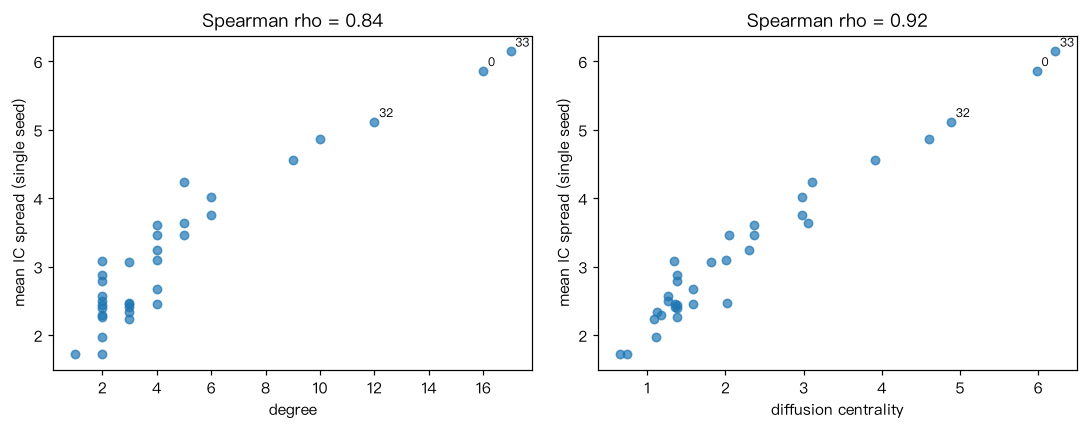
# 扩散中心性 DC = sum_{t=1..T} (q A)^t · 1。在空手道俱乐部网络上取 q=0.15, T=3，
# 与度中心性比较排名前 5 的节点；再用独立级联模型（每条边一次机会，概率 q）
# 模拟每个节点作为单种子的平均传播规模（200 次平均），用 Spearman 相关比较两种中心性与它的一致程度。
# 解读：两个相关系数越接近 1，说明该中心性越能预测单种子的传播能力。
import numpy as np
import networkx as nx
from scipy.stats import spearmanr

G = nx.karate_club_graph()
A = nx.to_numpy_array(G, weight=None)
n = A.shape[0]
q, Tmax = 0.15, 3

M = q * A
P = np.eye(n); S = np.zeros((n, n))
for _ in range(Tmax):          # 累加 M + M^2 + M^3
    P = P @ M
    S += P
DC = S @ np.ones(n)

def ic_spread(G, seed, q, rng):
    active, frontier = {seed}, [seed]
    while frontier:
        nxt = []
        for u in frontier:
            for v in G.neighbors(u):
                if v not in active and rng.random() < q:
                    active.add(v); nxt.append(v)
        frontier = nxt
    return len(active)

rng = np.random.default_rng(0)
spread = np.array([np.mean([ic_spread(G, s, q, rng) for _ in range(200)]) for s in range(n)])
deg = A.sum(1)
print("度 前5:", np.argsort(-deg)[:5].tolist())
print("DC 前5:", np.argsort(-DC)[:5].tolist())
print("IC 规模 前5:", np.argsort(-spread)[:5].tolist())
print("Spearman(度, IC) = %.3f" % spearmanr(deg, spread)[0])
print("Spearman(DC, IC) = %.3f" % spearmanr(DC, spread)[0])

import matplotlib.pyplot as plt
fig, (ax1, ax2) = plt.subplots(1, 2, figsize=(10, 4))
for ax, x, name in [(ax1, deg, "degree"), (ax2, DC, "diffusion centrality")]:
    ax.scatter(x, spread, s=30, c="tab:blue", alpha=0.7)
    for v in np.argsort(-spread)[:3]:
        ax.annotate(str(v), (x[v], spread[v]), fontsize=8, xytext=(3, 3), textcoords="offset points")
    ax.set_xlabel(name); ax.set_ylabel("mean IC spread (single seed)")
    ax.set_title("Spearman rho = %.2f" % spearmanr(x, spread)[0])
plt.tight_layout(); plt.show()