Example03 / 10
中心性稳定性——简化版病例删除 bootstrap
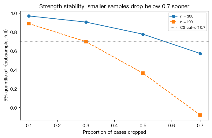
仿照 bootnet 的思路:从样本中无放回地保留 90%、70%、50%、30% 的被试,每个比例重复 100 次, 计算子样本强度与全样本强度的相关,取其 5% 分位数;CS 系数近似为该分位数仍 ≥ 0.7 时可删去的最大比例。 输出解读:保留比例越低,相关越低;n = 100 时 CS 明显低于 n = 300——小样本的中心性排序不可靠。 bootnet 的正式 CS 系数使用更细的删除比例、1000 次以上重抽样,并在每个子样本中重新选择正则化参数。
Output输出图
Output文字输出
n = 300: {'保留90%': 0.97, '保留70%': 0.9, '保留50%': 0.78, '保留30%': 0.57} → CS ≈ 0.5
n = 100: {'保留90%': 0.89, '保留70%': 0.7, '保留50%': 0.36, '保留30%': -0.08} → CS ≈ 0.1Code代码
# 仿照 bootnet 的思路:从样本中无放回地保留 90%、70%、50%、30% 的被试,每个比例重复 100 次,
# 计算子样本强度与全样本强度的相关,取其 5% 分位数;CS 系数近似为该分位数仍 ≥ 0.7 时可删去的最大比例。
# 输出解读:保留比例越低,相关越低;n = 100 时 CS 明显低于 n = 300——小样本的中心性排序不可靠。
# bootnet 的正式 CS 系数使用更细的删除比例、1000 次以上重抽样,并在每个子样本中重新选择正则化参数。
import numpy as np

TRUE_EDGES = {(0, 1): .40, (1, 5): .30, (1, 8): .25, (5, 8): .25, (2, 3): .40,
              (3, 6): .30, (3, 7): .20, (3, 4): .20, (0, 3): .20, (6, 7): .20}

def simulate_symptoms(n, seed=0):
    K = np.eye(9)                        # 模拟数据,仅用于演示方法
    for (i, j), w in TRUE_EDGES.items():
        K[i, j] = K[j, i] = -w
    rng = np.random.default_rng(seed)
    return rng.multivariate_normal(np.zeros(9), np.linalg.inv(K), size=n)

def strength_of(X):
    K = np.linalg.inv(np.cov(X, rowvar=False))
    d = np.sqrt(np.diag(K))
    P = -K / np.outer(d, d)
    np.fill_diagonal(P, 0)
    return np.abs(P).sum(axis=1)

def case_drop(X, keep_props=(0.9, 0.7, 0.5, 0.3), n_boot=100, seed=1):
    """返回 {保留比例: 子样本与全样本强度相关的 5% 分位数}。"""
    rng = np.random.default_rng(seed)
    s_full = strength_of(X)
    n = X.shape[0]
    out = {}
    for p in keep_props:
        cors = []
        for _ in range(n_boot):
            idx = rng.choice(n, int(p * n), replace=False)   # 无放回子抽样
            cors.append(np.corrcoef(strength_of(X[idx]), s_full)[0, 1])
        out[p] = np.quantile(cors, 0.05)
    return out

curves = {}                              # 记录各样本量的结果,供作图
for n in [300, 100]:
    res = case_drop(simulate_symptoms(n, seed=2))
    curves[n] = res
    cs = max([1 - p for p, q in res.items() if q >= 0.7], default=0.0)
    print(f"n = {n}:", {f"保留{int(p * 100)}%": round(float(q), 2) for p, q in res.items()},
          f"→ CS ≈ {cs:.1f}")

import matplotlib.pyplot as plt
fig, ax = plt.subplots(figsize=(6.4, 4.2))
for (n, res), mk, ls in zip(curves.items(), "os", ["-", "--"]):
    ax.plot([1 - p for p in res], list(res.values()), marker=mk, ls=ls, label=f"n = {n}")
ax.axhline(0.7, color="gray", ls=":", lw=1, label="CS cut-off 0.7")
ax.set(xlabel="Proportion of cases dropped", ylabel="5% quantile of r(subsample, full)",
       title="Strength stability: smaller samples drop below 0.7 sooner")
ax.legend(fontsize=8)
plt.tight_layout(); plt.show()Run在浏览器中运行
首次加载 Python 环境约需 20–40 秒;可以修改参数后重新运行。