Example06 / 14
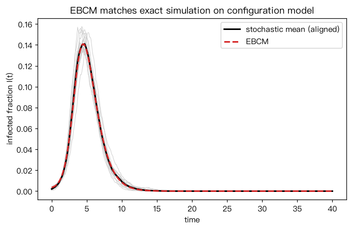
边基仓室模型(EBCM)与精确随机模拟的比较
Miller–Volz 边基模型把配置模型上的 SIR 化为一个关于 θ 的常微分方程:
dθ/dt = -β θ + β ψ’(θ)/
Output输出图
Output文字输出
大暴发次数:15 / 30
峰值 I:EBCM = 0.141,模拟 = 0.141
最终规模:EBCM = 0.607,均匀混合 ODE = 0.931
Code代码
# Miller–Volz 边基模型把配置模型上的 SIR 化为一个关于 θ 的常微分方程:
#   dθ/dt = -β θ + β ψ'(θ)/<k> + γ (1-θ),  S = ψ(θ),  dR/dt = γ I,  I = 1 - S - R
# 其中 ψ(x)=Σ P(k) x^k 是度分布的生成函数,θ 为“一条随机边尚未传来感染”的概率。
# 精确模拟用事件驱动法:每个感染者的恢复时间 ~ Exp(γ),沿每条边的传播时间 ~ Exp(β),
# 只有传播时间早于恢复时间才发生传播(与连续时间马尔可夫 SIR 同分布)。
# 解读:对大规模配置模型,EBCM 曲线与随机模拟的平均曲线(按暴发时刻对齐后)几乎重合;
#       同一参数下,均匀混合 ODE(R0 = β<k>/γ)会高估峰值与最终规模。
import heapq
import numpy as np
import networkx as nx
from scipy.integrate import solve_ivp

rng = np.random.default_rng(0)
N = 5000
deg_seq = rng.choice([2, 3, 4, 10], size=N, p=[0.35, 0.3, 0.25, 0.1])
if deg_seq.sum() % 2:
    deg_seq[0] += 1
G = nx.Graph(nx.configuration_model(deg_seq, seed=0))
G.remove_edges_from(nx.selfloop_edges(G))
beta, gamma = 0.8, 1.0

def fast_sir(G, beta, gamma, seed, rng, tmax=40):
    status = {}
    rec_time = {}
    pq = [(0.0, "inf", seed)]
    times, counts = [], []
    S, I, R = G.number_of_nodes(), 0, 0
    while pq:
        t, ev, v = heapq.heappop(pq)
        if t > tmax:
            break
        if ev == "inf":
            if status.get(v, "S") != "S":
                continue
            status[v] = "I"; S -= 1; I += 1
            rec_time[v] = t + rng.exponential(1 / gamma)
            heapq.heappush(pq, (rec_time[v], "rec", v))
            for u in G.neighbors(v):
                if status.get(u, "S") == "S":
                    tt = t + rng.exponential(1 / beta)
                    if tt < rec_time[v]:
                        heapq.heappush(pq, (tt, "inf", u))
        else:
            status[v] = "R"; I -= 1; R += 1
        times.append(t); counts.append((S, I, R))
    return np.array(times), np.array(counts) / G.number_of_nodes()

k = np.array([d for _, d in G.degree()]); vals, cnt = np.unique(k, return_counts=True); P = cnt / cnt.sum()
kmean = (vals * P).sum()
psi = lambda x: (P * x**vals).sum()
dpsi = lambda x: (P * vals * x**(vals - 1)).sum()
eps = 1e-3
def rhs(t, y):
    th, R = y
    S = psi(th); I = 1 - S - R
    return [-beta * th + beta * dpsi(th) / kmean + gamma * (1 - th), gamma * I]
tgrid = np.linspace(0, 40, 401)
sol = solve_ivp(rhs, (0, 40), [1 - eps, 0.0], t_eval=tgrid, rtol=1e-8)
I_ebcm = 1 - np.array([psi(t) for t in sol.y[0]]) - sol.y[1]

# 随机模拟:只保留发生大暴发的轨迹,并按 I 达到 1% 的时刻与 EBCM 对齐
t_ebcm_1 = tgrid[np.argmax(I_ebcm > 0.01)]
curves = []
for r in range(30):
    t, c = fast_sir(G, beta, gamma, int(rng.integers(N)), rng)
    if c[-1, 2] > 0.1:
        t0 = t[np.argmax(c[:, 1] > 0.01)]
        curves.append(np.interp(tgrid, t - t0 + t_ebcm_1, c[:, 1], left=0, right=0))
I_sim = np.mean(curves, axis=0)
R0_hom = beta * kmean / gamma
r_hom = 1 - np.exp(-R0_hom)  # 迭代求均匀混合最终规模
for _ in range(200):
    r_hom = 1 - np.exp(-R0_hom * r_hom)
print("大暴发次数:%d / 30" % len(curves))
print("峰值 I:EBCM = %.3f,模拟 = %.3f" % (I_ebcm.max(), I_sim.max()))
print("最终规模:EBCM = %.3f,均匀混合 ODE = %.3f" % (1 - psi(sol.y[0][-1]), r_hom))

import matplotlib.pyplot as plt
fig, ax = plt.subplots(figsize=(6.4, 4.2))
for c in curves:
    ax.plot(tgrid, c, c="0.8", lw=0.6)
ax.plot(tgrid, I_sim, "k-", lw=2, label="stochastic mean (aligned)")
ax.plot(tgrid, I_ebcm, "--", c="tab:red", lw=2, label="EBCM")
ax.set_xlabel("time"); ax.set_ylabel("infected fraction I(t)"); ax.legend()
ax.set_title("EBCM matches exact simulation on configuration model")
plt.tight_layout(); plt.show()Run在浏览器中运行
首次加载 Python 环境约需 20–40 秒;可以修改参数后重新运行。