活动驱动时间网络上的 SIS 阈值

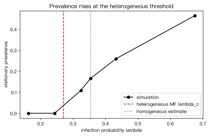
# 活动驱动模型（Perra 等 2012）：每个时间步，节点 i 以概率 a_i 被激活，向 m 个随机节点发出接触，
# 接触只持续一个时间步。感染者每步以概率 μ 恢复，每次 S–I 接触以概率 λ 传播。
# 线性化平均场（推导见“数学推导与算法”D 节）给出阈值 λ_c = μ / [m(<a> + sqrt(<a^2>))]；
# 若忽略活动性的异质性（人人活动性都取 <a>），阈值为 μ / (2m<a>)，更高。
# 解读：模拟的稳态流行率在异质理论阈值附近开始离开 0，低于“同质”估计——活跃个体既常感染别人也常被感染。
import numpy as np

rng = np.random.default_rng(1)
N, m, mu, steps = 5000, 1, 0.1, 1500
a = np.where(rng.random(N) < 0.2, 0.5, 0.05)          # 20% 高活跃个体
lam_c = mu / (m * (a.mean() + np.sqrt((a**2).mean())))
lam_hom = mu / (2 * m * a.mean())
print("<a> = %.3f, sqrt(<a^2>) = %.3f" % (a.mean(), np.sqrt((a**2).mean())))
print("异质平均场 λ_c = %.3f；忽略活动异质性的估计 = %.3f" % (lam_c, lam_hom))

def simulate(lam, rng):
    inf = np.zeros(N, bool); inf[rng.choice(N, 250, replace=False)] = True
    prev = []
    for t in range(steps):
        src = np.repeat(np.flatnonzero(rng.random(N) < a), m)
        dst = rng.integers(N, size=src.size)
        new = np.zeros(N, bool)
        for u, v in ((src, dst), (dst, src)):          # 接触是双向的
            hit = inf[u] & ~inf[v] & (rng.random(u.size) < lam)
            new[v[hit]] = True
        inf = (inf & ~(rng.random(N) < mu)) | new
        if t >= steps - 500:
            prev.append(inf.mean())
        if not inf.any():
            return 0.0
    return float(np.mean(prev))

lams, prevs = [0.6 * lam_c, 0.9 * lam_c, 1.2 * lam_c, 1.6 * lam_c, lam_hom, 2.5 * lam_c], []
for lam in lams:
    prevs.append(simulate(lam, rng))
    print("λ = %.3f (= %.1f λ_c)  稳态流行率 = %.4f" % (lam, lam / lam_c, prevs[-1]))

import matplotlib.pyplot as plt
fig, ax = plt.subplots(figsize=(6.4, 4.2))
order = np.argsort(lams)
ax.plot(np.array(lams)[order], np.array(prevs)[order], "ko-", label="simulation")
ax.axvline(lam_c, ls="--", c="tab:red", label="heterogeneous MF lambda_c")
ax.axvline(lam_hom, ls=":", c="0.4", label="homogeneous estimate")
ax.set_xlabel("infection probability lambda"); ax.set_ylabel("stationary prevalence"); ax.legend()
ax.set_title("Prevalence rises at the heterogeneous threshold")
plt.tight_layout(); plt.show()